Xiangyu Zhang, Xinyu Zhou, Mengxiao Lin, Jian Sun; Proceedings of the IEEE Conference on Computer Vision and Pattern Recognition (CVPR), 2018, pp. 6848-6856, 2017 ShuffleNet: An Extremely Efficient Convolutional Neural Network for Mobile Devices
위 논문은 2017년도에 작성되었으며 2018년에 CVPR에서 발표되었다.
논문에서 제안하는 pointwise group convolution과 channel shuffle에 대해서 자세히 살펴본다.
We introduce an extremely computation efficient CNN architecture named ShuffleNet, designed specially for mobile devices with very limited computing power.
우리는 효과적인 연산량을 가진 CNN 아키쳐 기반의 ShuffleNet을 소개한다. 이 아키텍처는 매우 효과제한적인 computing power를 요구하는 모바일 장치를 target으로 설계되었다.
The new architecture utilizes two proposed operations, pointwise group convolution and channel shuffle, to greatly reduce computation cost while maintaining accuracy.
논문에서 제안하는 아키텍처는 성능은 유지하면서 computation cost을 크게 줄이기 위해 pointwise group convolution과 channel shuffle을 활용한다.
Experiments on ImageNet classification and MS COCO object detection demonstrate the superior performance of ShuffleNet over other structures, e.g. lower top-1 error (absolute 6.7%) than the recent MobileNet system on ImageNet classification under the computation budget of 40 MFLOPs.
ImageNet classification, MS COCO object detection의 실험에서 ShuffleNet은 다른 모델에 비해서 우수한 성능을 보여준다. 예를들어 최근 ImageNet classification에서 40MLFLOPS의 이하 연산량의 시스템을 가진 MobileNet보다 top-1에서 더 낮은 에러율(6.7%)를 보였다.
Introduction
background research
The last few years have seen the success of deep neural networks in computer vision tasks, in which model designs play an important role. The increasing needs of running high quality deep neural networks on embedded devices encourage the study on efficient model designs.
지난 몇 년 동안 컴퓨터 비전 작업에서 deep neural network는 많은 발전을 이루었다. 임베디드 장치에서 높은 품질의 deep neural networks를 실행해야 하는 필요성이 증가함에 따라 효율적인 모델 설계에 대한 연구가 촉진되었다.
recent research
This report examines the opposite extreme: pursuing the best accuracy in very limited computational budgets at tens or hundreds of MFLOPs, focusing on common mobile platforms such as drones, robots, and phones.
트렌드와는 반대로 우리는 드론, 로봇 및 휴대폰과 같은 일반적인 모바일 플랫폼에 초점을 맞춘 수십 또는 수백 개 연산량이 제한된 computational cost를 가지고 높은 성능을 낼 수 있는 모델을 고안한다.
propose
We propose using pointwise group convolutions instead to reduce computation complexity.
우리는 계산 복잡도를 줄이기 위해 pointwise group convolutions을 사용한다.
To overcome the side effects brought by pointwise group convolutions, we come up with a novel channel shuffle operation to help the information flowing across feature channels.
pointwise group convolutions의 단점을 극복하기 위해, 우리는 특징을 가지고 있는 채널 간의 정보를 교환하기 위해 channel shuffle 개념을 제안한다.
Based on the two techniques, we build a highly efficient architecture called ShuffleNet. Compared with popular structures like, for a given computation complexity budget, our ShuffleNet allows more feature map channels, which helps to encode more information and is especially critical to the performance of very small networks.
pointwise group convolutions과 channel shuffle을 기반으로 우리는 매우 효율적인 아키텍처를 설계했고 적은 layer로 구성된 small Network에서도 높은 성능을 내기 위해 특징 정보를 encoding하는 feature map channel을 더 많이 사용할 수 있게 되었다.
We evaluate our models on the challenging ImageNet classification and MS COCO object
detection tasks.
ImageNet Classification과 MS COCO object detection task에서 우리의 성능을 테스트했다.
Compared with the state-of-the-art architecture MobileNet, ShuffleNet achieves superior performance by a significant margin, e.g.absolute 6.7% lower ImageNet top-1 error at level of 40 MFLOPs.
SOTA인 MobileNet과 비교하면 ShuffleNet이 40 MFLOP 수준에서 ImageNet top-1 error가 6.7% 감소하는 등 상당한 차이로 우수한 성능을 달성한다.
Summary
위 논문서는 MobileNet에 적용된 Pointwise convolution도 많은 연산량을 요구한다는 것을 발견해서 Pointwise group convolution을 사용한다. 그러나 group convolution이 가진 단점때문에 각 채널간의 정보 교환이 잘 이뤄지지 않는다. 이를 해결기위해 논문에서는 channel shuffle을 통해 단점을 보완하고자 한다.
Related Work
Efficient Model Designs
For example, GoogLeNet increases the depth of networks with much lower complexity compared to simply stacking convolution layers.
GoogleLeNet은 낮은 복잡도로 convolution layers를 쌓아 네트워크의 깊이를 증가시킨다.
SqueezeNet reduces parameters and computation significantly while maintaining accuracy.
SqueezeNet은 모델의 성능을 유지하면서 parameters와 computation을 크게 줄인다.
ResNet utilizes the efficient bottleneck structure to achieve impressive performance.
ResNet은 효율적인 bottleneck structure를 활용하여 뛰어난 성능을 달성한다.
The concept of group convolution, which should be first introduced in AlexNet for distributing the model over two GPUs, has shown the potential to improve accuracy in.
AlexNet에서 도입된 두 개의 GPU를 사용하여 분산학습 하는 group convolution은 정확도를 향상시킬 수 있는 가능성을 보여주었다.
Depthwise separable convolution proposed in Xception generalizes the ideas of separable convolutions in Inception series.
Xception에서 제안된 Depthwise separable convolution은 Inception에서 제안된 separable convolutions 아이디어를 통해 더 확장되었다.
Recently, MobileNet utilizes the depthwise separable convolutions and gains state-of-the-art results among lightweight models.
최근 MobileNet은 depthwise separable convolutions활용하여 경량화된 model에서 높은 성능을 냈다.
Our work generalizes group convolution and depthwise separable convolution in a novel
form.
우리는 group convolution과 depthwise separable convolution을 통해 모델을 확장한다.
Model Acceleration
This direction aims to accelerate inference while preserving accuracy of
a pretrained model.
pretrained model의 성능은 유지하면서 inference를 더 빠르게 하는 것을 목표로 한다.
Pruning network connections or channels reduces redundant connections in a pre-trained model while maintaining performance.
네트워크 연결을 줄이거나 채널을 줄이는 것은 성능은 유지하면서 사전학습된 모델의 불필요한 연산을 줄인다.
Quantization and factorization are proposed in literature to reduce redundancy in calculations to speed up inference.
계산의 중복성을 줄이고 추론을 가속화하기 위해 Quantization와 factorization이 제안된다.
Without modifying the parameters, optimized convolution algorithms implemented by FFT(Fast Fourier Transform) and other methods decrease time consumption in practice.
parameters를 수정하지 않고 FFT(Fast Fourier Transform) 및 다른 방법으로 구현된 최적화된 convolution algorithms을 사용하면 학습 시간이 줄어든다.
Distilling transfers knowledge from large models into small ones, which makes training small models easier.
Distilling은 큰 모델에서 작은 모델로 지식을 전달하여 작은 모델의 훈련을 쉽게 만든다.
모델 디스틸링(Model Distillation)은 큰 모델(일반적으로는 성능이 좋지만 크기가 크고 계산 비용이 높은 모델)에서 작은 모델로 지식을 전달하는 방법으로 작은 모델도 큰 모델과 유사한 성능을 달성할 수 있게 한다.
Compared to these methods, our approach focuses on better model designs to improve performance rather than accelerating or transferring an existing model.
우리의 접근법은 앞서 소개한 방법들, 기존 모델을 가속화하거나 잘 전달(transferring)하는 것이 아니라 성능을 향상시키기 위해 더 나은 모델 설계에 초점을 맞춘다.
Approach
Channel Shuffle for Group Convolutions
Modern convolutional neural networks usually consist of repeated building blocks with the same structure.
현대의 convolutional neural networks는 반복적인 구조으로 구성된다.
Among them, state-of-the-art networks such as Xception and ResNeXt introduce efficient depthwise separable convolutions or group convolutions into the building blocks to strike an excellent trade-off between representation capability and computational cost.
그 중 Xception 및 ResNeXt와 같은 SOTA 모델은 효율적인 depthwise separable convolutions 또는 group convolutions을 네트워크 구조에 도입하여 representation capability과 computational cost 사이의 우수한 균형을 달성한다.
However, we notice that both designs do not fully take the 1 × 1 convolutions (also called pointwise convolutions) into account, which require considerable complexity.
그러나 두 모델 전부 상당한 계산 복잡도를 요하는 1×1conv(pointwise convolutions)에 대해서는 고려하지 않는다는 것을 알게 되었다.
For example, in ResNeXt only 3 × 3 layers are equipped with group convolutions. As a result, for each residual unit in ResNeXt the pointwise convolutions occupy 93.4% multiplication-adds (cardinality = 32).
예를 들어 ResNeXt에서는 3 × 3 layers에만 group convolutions 적용된다. 결과적으로 ResNeXt의 각 residual unit(skip connection)에 대해 pointwise convolutions은 93.4%의 multiplication-adds를 차지한다.
(깊이 = 32).
In tiny networks, expensive pointwise convolutions result in limited number of channels to meet the complexity constraint, which might significantly damage the accuracy.
작은 네트워크(tiny networks)에서 많은 연산을 요하는 pointwise convolutions은 complexity constraint을 충족하기 위해 채널 수를 제한하면 성능 향상에 영향이 갈 수 있다.
To address the issue, a straightforward solution is to apply channel sparse connections, for example group convolutions, also on 1 × 1 layers.
이 문제를 해결하기 위해 간단한 해결책은 예를 들어 채널에 sparse connections적용(group convolutions을 1x1 layer에도 적용하는 것)하는 것이다.
By ensuring that each convolution operates only on the corresponding input channel group, group convolution significantly reduces computation cost.
각 convolution이 입력 채널의 그룹에서만 작동하도록 함으로써 group convolution은 계산 비용을 크게 절감한다.
However, if multiple group convolutions stack together, there is one side effect: outputs from a certain channel are only derived from a small fraction of input channels.
그러나 여러 group convolutions 함께 쌓이면 한 가지 부작용이 있는데 특정 채널의 출력은 입력 채널의 극히 일부에서만 도출다. 이 문장이 무슨뜻인지 아래 자세히 설명하겠다.
input channel들이 여러 그룹으로 나누어지고, 각 그룹 내의 채널들만이 해당 그룹의 출력 채널을 계산하는 데 사용된다는 것이다.
예를 들어, input channel이 16개 있고 그룹 수가 4라면, 각 그룹은 4개의 input channel을 가지게 된다. 이 경우, 각 출력 채널은 해당 그룹의 4개 input channel만을 사용하여 계산되며, 다른 그룹의 input channel은 사용되지 않는다. 따라서, 각 출력 채널은 전체 input channel중 일부분만을 사용하여 계산되는 것이다.
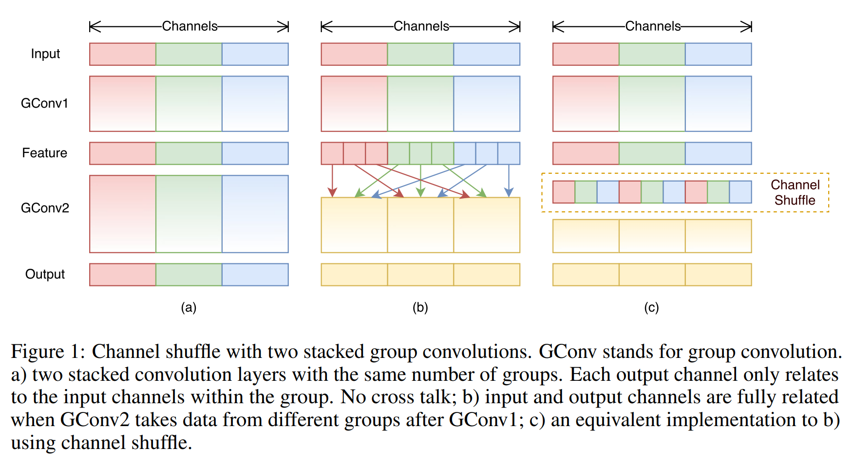
Fig 1 (a) illustrates a situation of two stacked group convolution layers. It is clear that outputs from a certain group only relate to the inputs within the group.
Fig 1(a)는 두 개의 적층된group convolution layers의 상황을 보여준다. 특정 그룹의 출력은 그룹 내 입력에만 관련되어 있음을 설명한다.
This property blocks information flow between channel groups and weakens representation.
이런 특성은 channel groups 간의 정보 흐름을 차단하고 feature representation을 약화시킨다.
If we allow group convolution to obtain input data from different groups (as shown in Fig 1 (b)), the input and output channels will be fully related.
만약 group convolution이 different groups으로부터 입력 데이터를 얻을 수 있도록 허용한다면, (그림 1 (b)) 입력 및 출력 채널은 서로 잘 관련되어 있게 된다.
Specifically, for the feature map generated from the previous group layer, we can first divide the channels in each group into several subgroups, then feed each group in the next layer with different subgroups.
특히, 이전 group layer에서 생성된 feature map의 경우 먼저 채널을 각 group별로 나눈다음 다음 계층의 입력에 서로 다른 하위 group을 전파할 수 있다.
This can be efficiently and elegantly implemented by a channel shuffle operation (Fig 1 (c))
이는 channel shuffle 작업을 통해 효율적이고 우아하게 구현될 수 있다.(그림 1(c)).
Groups whose output has g × n channels; we first reshape the output channel dimension into (g, n), transposing and then flattening it back as the input of next layer.
출력이 g × n개의 채널을 갖는 그룹의 출력 채널 차원을 (g, n)로 바꾸고 이를 transpose한 후(n, g) 다음 레이어의 입력으로 flattening한다.(n x g)
Note that the operation still takes effect even if the two convolutions have different numbers of groups.
두 convolutions의 그룹 수가 서로 다른 경우에도 효과가 있다.
Moreover, channel shuffle is also differentiable, which means it can be embedded into network structures for end-to-end training.
게다가, channel shuffle은 미분 가능함으로 네트워크 구조에 포함되어 end-to-end 훈련이 가능하다는 것을 의미한다.(역전파 학습방식 때문)
Channel shuffle operation makes it possible to build more powerful structures with multiple group convolutional layers.
group convolutional layers에 Channel shuffle을 통해 성능이 좋은 네트워크를 구축하게 한다.
In the next subsection we will introduce an efficient network unit with channel shuffle and group convolutions.
다음 절에서는 channel shuffle과 group convolutions이 있는 효율적인 네트워크를 소개한다.
ShuffleNet Unit
Taking advantage of the channel shuffle operation, we propose a novel ShuffleNet unit specially
designed for small networks.
channel shuffle을 이용하여, small network로 설계된 ShuffleNet을 제안한다.
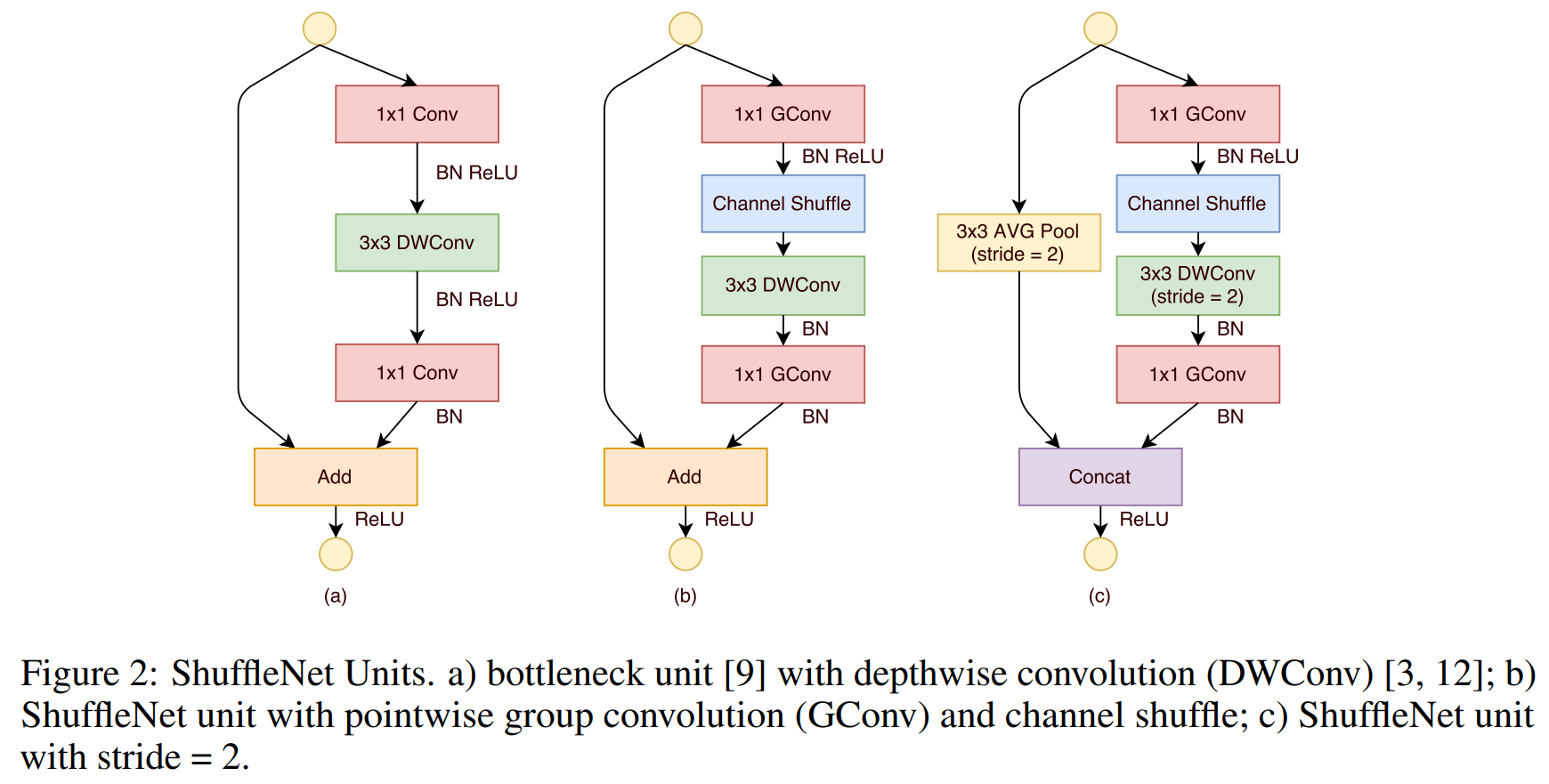
We start from the design principle of bottleneck unit in Fig 2 (a).
우리는 그림 2(a)의 bottleneck의 구조에서 시작한다.
It is a residual block. In its residual branch, for the 3 × 3 layer, we apply a computational economical 3 × 3 depthwise convolution on the bottleneck feature map.
residual block에서 bottleneck의 3×3 layer에 대한 feature map을 구하는데 있어 효율적인 계산을 위해 3×3 depthwise convolution을 적용한다.
Then, we replace the first 1 × 1 layers with pointwise group convolution followed by a channel shuffle operation, to form a ShuffleNet unit, as shown in Fig 2 (b).
그런 다음 첫 번째 1×1 layers를 pointwise group convolution에 channel shuffle 적용한다. 그림 2 (b)와 같이 ShuffleNet 유닛을 형성한다.
The purpose of the second pointwise group convolution is to recover the channel dimension to match the shortcut path.
두 번째 pointwise group convolution의 목적은 shortcut path와 차원이 일치하도록 dimension을 복구하는 것이다.
For simplicity, we do not apply an extra channel shuffle operation after the second pointwise layer.
심플함을 위해 두 번째 pointwise layer이후에 channel shuffle을 추가로 적용하지 않는다.
As for the case where ShuffleNet is applied with stride, we simply make two modifications (see Fig 2 (c)): (i) add a 3 × 3 average pooling on the shortcut path; (ii) replace the element-wise addition with channel concatenation, which makes it easy to enlarge channel dimension with little extra computation cost.
ShuffleNet에 stride가 적용되는 경우는 (i) shortcut path에 3×3 average pooling 추가한다, (ii) 요소별 추가를 채널 연결로 대체하여 추가 계산 비용 없이 채널 차원을 쉽게 확장할 수 있습니다(그림 2(c) 참조). element-wise addition(요소별 덧셈)을 channel concatenation(채널 연결)로 대체하면, 추가적인 계산 비용이 거의 없이 채널 차원을 쉽게 확장할 수 있다.
Thanks to pointwise group convolution with channel shuffle, all components in ShuffleNet unit can be computed efficiently.
pointwise group convolution에 channel shuffle을 사용하여 ShuffleNet의 layer들을 효율적으로 계산할 수 있다.
Compared with ResNet(bottleneck design) and ResNeXt, our structure has less complexity under the same settings.
ResNet및 ResNeXt와 비교하면 동일한 설정에서 구조가 덜 복잡하다.
For example, given the input size c × h × w and the bottleneck channels m, ResNet unit requires hw(2cm + 9m^2) FLOPs and ResNeXt has hw(2cm + 9m2/g) FLOPs, while our ShuffleNet unit requires only hw(2cm/g + 9m) FLOPs, where g means the number of groups for convolutions.
예를 들어, 입력 크기 c × h × w와 bottleneck channels를 m으로 하면 ResNet는 hw(2cm + 9m^2) FLOP가 필요하고 ResNeXt에는 hw(2cm + 9m2/g) FLOP가 필요한 반면 ShuffleNet는 hw(2cm/g + 9m) FLOP만 필요하다. (g는 컨볼루션을 위한 그룹의 수를 의미함)
In other words, given a computational budget, ShuffleNet can use wider feature maps.
다시 말해, computational budget에서 ShuffleNet은 더 넓은 feature maps을 사용할 수 있다.
We find this is critical for small networks, as tiny networks usually have an insufficient number of channels to pass the information.
small networks에는 일반적으로 정보를 전달할 수 있는 채널 수가 충분하지 않기 때문에 더 넓은 feature map을 사용하는 것은 중요하다.
In addition, in ShuffleNet depthwise convolution only performs on bottleneck feature maps.
Even though depthwise convolution usually has very low theoretical complexity, we find it difficult to efficiently implement on low-power mobile devices, which may result from a worse computation/memory access ratio compared with other dense operations.
depthwise convolution은 이론적으로 complexity가 낮지만, 저전력 모바일 장치에서 효율적으로 실행되기가 어렵다는 것을 알게 되었다 그리고 다른 dense layer연산에 비해 비 효율적인 계산/메모리 액세스가 발생한다.
In ShuffleNet units, we intentionally use depthwise convolution only on bottleneck in order to prevent overhead as much as possible.
따라서 ShuffleNet 장치에서는 오버헤드를 최대한 방지하기 위해 bottleneck에만depthwise convolution을 사용한다.
Network Architecture
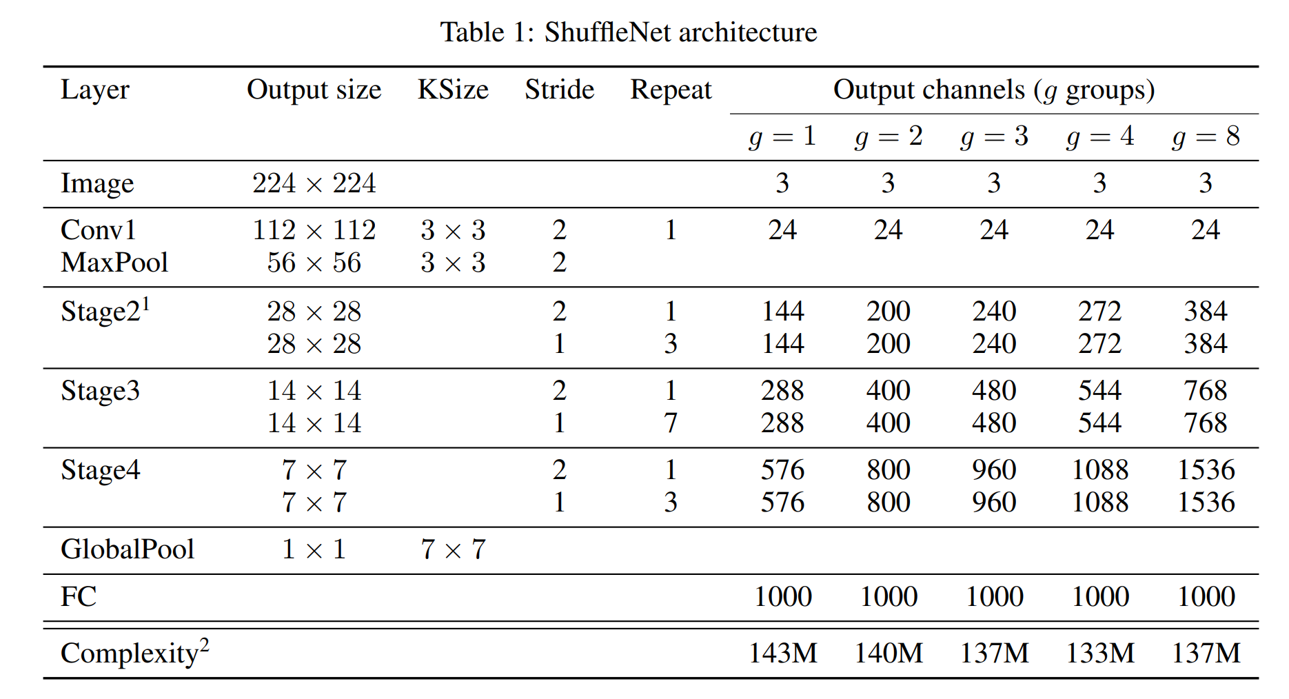
Built on ShuffleNet units, we present the overall ShuffleNet architecture in Table 1.
ShuffleNet 아키텍처를 표 1에 제시한다.
The proposed network is mainly composed of a stack of ShuffleNet units grouped into three stages.
제안된 네트워크는 주로 3 단계로 나뉘어진 ShuffleNet으로 구성된다.
The first building block in each stage is applied with stride = 2.
각 단계의 첫 번째 block은 stride = 2로 적용된다.
Other1 within a stage stay the same, and for the next stage the output channels are doubled.
같은 단계의 hyper-parameters 는 동일하게 유지되며, 다음 단계에서는 출력 채널이 두 배가 된다.
we set the number of bottleneck channels to 1/4 of the output channels for each ShuffleNet unit.
각 ShuffleNet에 대한 bottleneck channels를 출력 채널의 1/4로 설정했다.
Our intent is to provide a reference design as simple as possible, although we find that further hyper-parameter tunning might generate better results.
우리의 의도는 설계를 가능한 한 단순하게 하는 것이지만, 추가적인 hyper-parameter tunning이 더 나은 결과를 생성할 수 있다는 것을 발견했다.
In ShuffleNet units, group number g controls the connection sparsity of pointwise convolutions.
ShuffleNet에서 group 갯수 g는 pointwise convolutions의 connection sparsity을 제어한.
connection sparsity
신경망의 특정 뉴런이나 레이어 간에 연결이 없거나, 또는 연결이 적게 설정되어 있음을 의미한다.
Table 1 explores different group numbers and we adapt the output channels to ensure overall computation cost roughly unchanged (~140 MFLOPs).
표 1은 다양한 group 갯수에 따라 전체 계산 비용이 거의 변하지 않도록 출력 채널을 한다(~140 MFLOP).
Obviously, larger group numbers result in more output channels (thus more convolutional filters) for a given complexity constraint, which helps to encode more information, though it might also lead to degradation for an individual convolutional filter due to limited corresponding input channels.
명백히, 더 큰 그룹 수는 주어진 복잡성 제약에 대해 더 많은 출력 채널(따라서 더 많은 컨볼루션 필터)을 결과로 가져오며, 이는 더 많은 정보를 인코딩하는 데 도움이 되지만, 한편으로는 해당 입력 채널이 제한적이기 때문에 개별 컨볼루션 필터의 성능 저하를 초래할 수도 있다.
In Sec 4.1.1 we will study the impact of this number subject to different computational constrains.
4.1.1절에서 우리는 다른 computational constrains에 따라 이 숫자(group 갯수)의 영향을 연구한다.
To customize the network to a desired complexity, we can simply apply a scale factor s on the number of channels.
원하는 task에 따라 complexity를 customizing하려면 채널 수에 스케일 팩터 s를 적용하면 된다.
For example, we denote the networks in Table 1 as "ShuffleNet 1×", then "ShuffleNet
s×" means scaling the number of filters in ShuffleNet 1× by s times thus overall complexity will be roughly s 2 times of ShuffleNet 1×.
"ShuffleNet 1×"는 기본 버전의 ShuffleNet을 의미하며, "ShuffleNet s×"는 기본 버전의 필터 수를 s배로 늘린 버전을 의미한다.
Experiments
We mainly evaluate our models on the ImageNet 2016 classification dataset.
우리는ImageNet 2016 classification dataset에서 모델을 평가한다.
We use our self-developed system for training, and follow most of the training settings and hyper-parameters used in, with two exceptions: (i) we set the weight decay to 4e-5 instead of 1e-4; (ii) we use slightly less aggressive scale augmentation for data preprocessing. Similar modifications are also referenced in because such small networks usually suffer from underfitting rather than overfitting.
우리는 자체 개발 시스템을 훈련에 사용하고, 대부분의 훈련에 설정된 hyper-parameters를 따르지만, 두 가지 예외가 있다. (i) weight decay를 1e-4가 아닌 4e-5로 설정한다. (ii) 데이터 전처리를 에서 less aggressive scale augmentation를 사용한다.이러한 수정사항들은 작은 네트워크들이 과적합보다는 과소적합에서 더 자주 고통받기 때문이다.
To benchmark, we compare single crop top-1 performance on ImageNet validation set, i.e. cropping 224 × 224 center view from 256× input image and evaluating classification accuracy.
benchmark를 위해 ImageNet validation set에서 single crop 상위 1위와 성능을 비교한다. 즉, 256배 입력 이미지에서 center crop을 적용해 224×224를 통해 정확도를 평가한.
Ablation Study
The core idea of ShuffleNet lies in pointwise group convolution and channel shuffle operation
referenced in Sections
ShuffleNet의 핵심 아이디어는 pointwise group convolution과 channel shuffle작동에 있다.
On the Importance of Pointwise Group Convolutions
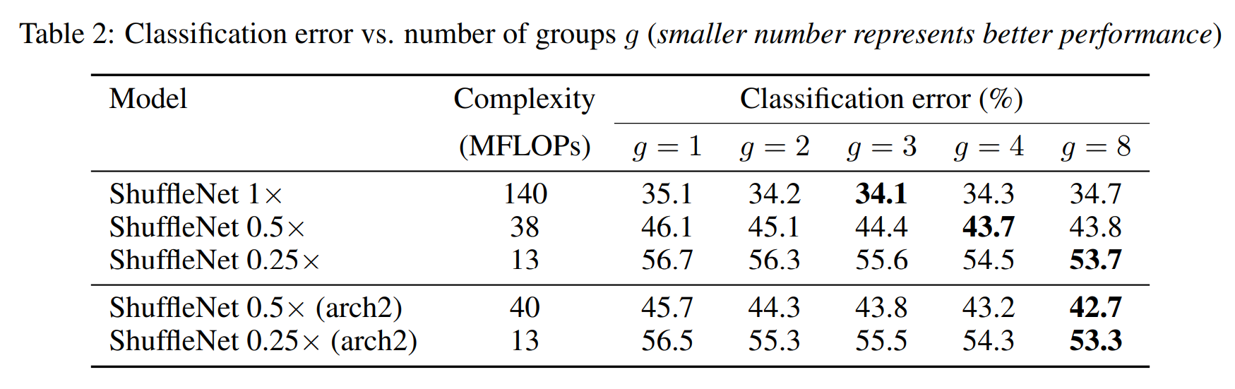
To evaluate the importance of pointwise group convolutions, we compare ShuffleNet models of the same complexity whose numbers of groups range from 1 to 8.
pointwise group convolutions의 중요성을 평가하기 위해, 우리는 groups 갯수를 1~8 로 변경하면서 ShuffleNet 모델을 비교한다.
If the group number equals 1, no pointwise group convolution is involved and then the ShuffleNet unit becomes an "Xception-like" structure.
group 갯수가 1이면 pointwise group convolution이 포함되지 않으며 ShuffleNet는 Xception과 유사한 구조를 갖는다.
For better understanding, we also scale the width of the networks to 3 different complexities
and compare their classification performance respectively.
더 나은 이해를 위해, 네트워크의 폭을 3가지 다른 복잡성으로 확장하고 성능을 각각 비교한다.
Results are shown in Table 2. From the results, we see that models with group convolutions (g > 1) consistently perform better than the counterparts without pointwise group convolutions (g = 1).
결과는 표 2에 나와 있다. 결과로부터, 우리는 group convolutions(g > 1)이 있는 모델이 pointwise group convolutions(g = 1)이 없는 모델보다 일관되게 더 나은 성능을 보인다는 것을 알 수 있다.
Smaller models tend to benefit more from groups. For example, for ShuffleNet 1× the best entry (g = 3) is 1.0% better than the counterpart, while for ShuffleNet 0.5× and 0.25× the gaps become 2.4% and 3.0% respectively.
모형이 작을수록 groups 갯수에 대해서 더 많은 혜택을 받는 경향이 있다. 예를 들어 ShuffleNet 1x 모델중 g = 3경우가 g=1일때 보다 1.0% 더 나은 반면 ShuffleNet 0.5x 및 0.25x의 경우 간격이 각각 2.4% 및 3.0%가 된다.
Note that group convolution allows more feature map channels for a given complexity constraint, so we hypothesize that the performance gain comes from wider feature maps which help to encode more information.
group convolution은 주어진 complexity constraint에 대해 더 많은 feature map채널을 허용하므로, 많은 정보를 encoding하는 wider한 feature map으로 부터 성능이 향상된다고 가정한다.
In addition, a smaller network involves thinner feature maps, meaning it benefits more from enlarged feature maps.
또한 작은 네트워크에는 thinner feature maps이 존재하는데 이는 enlarged feature maps에서 더 많은 이점을 얻을 수 있다.
Table 2 also shows that for some models (e.g. ShuffleNet 1×) when group numbers become relatively large (e.g. g = 4 or 8), the classification score saturates or even drops.
표 2는 또한 일부 모델(예: ShuffleNet 1×)의 경우 group 갯수가 상대적으로 커질 때(예: g = 4 또는 8) classification score가 saturates되거나 감소한다.
With an increase in group number (thus wider feature maps), input channels for each convolutional filter become fewer, which may harm representation capability.
group 갯수가 증가함에 따라(따라서wider feature maps) 각 convolutional filter에 대한 입력 채널이 적어지며, 이는 representation capability을 손상시킬 수 있다.
Interestingly, we also notice that for smaller models such as ShuffleNet 0.25× larger group numbers tend to better results consistently, which suggests wider feature maps are especially important for smaller models.
Inspired by this, for low-cost models we slightly modify the architecture in Table 1: we remove two units in Stage3 and widen each feature map to maintain the overall complexity.
이에 영감을 받아 low-cost models을 위해 표 1의 아키텍처를 약간 수정한다. Stage3에서 두 개의 유닛을 제거하고 각 feature map을 확장하여 전반적인 complexity 유지한다.
Results of the new architecture (named "arch2") are shown in Table 2.
새로운 아키텍처("arch2"라는 이름)의 결과는 표 2에 나와 있다.
It is clear that the newly designed models are consistently better than the counterparts; besides, pointwise group convolution still takes effect in the architecture.
새로 설계된 모델이 다른 모델보다 일관되게 더 낫다는 것을 설명한다. 게다가, pointwise group convolution은 네트워크에서 여전히 효과적이다.
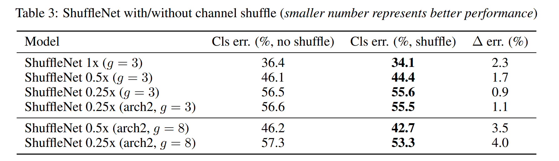
Channel Shuffle vs. No Shuffle
The purpose of shuffle operation is to enable cross-group information flow for multiple group
convolution layers.
channel shuffle의 목적은 여러 group convolution layer에 대해 grouped된 channel의 정보 흐름을 활성화하는 것이다.
Table 3 compares the performance of ShuffleNet structures (group number is set to 3 or 8 for instance) with/without channel shuffle.
표 3은 channel shuffle을 사용하거나 사용하지 않는 ShuffleNet structures(예: group 갯수가 3 또는 8로 설정됨)의 성능을 비교한다.
The evaluations are performed under three different scales of complexity.
평가는 세 가지 다른 복잡성을 가지는 모델로 수행된다.
It is clear that channel shuffle consistently boosts classification scores for different settings.
channel shuffle은 다양한 설정에 대한 classification scores를 지속적으로 높여준다.
Especially, when group number is relatively large (e.g. g = 8), models with channel shuffle outperform the counterparts by a significant margin, which shows the importance of cross-group information interchange.
특히 group 갯수가 상대적으로 클 때(예: g = 8) channel shuffle이 있는 모델이 없는 모델보다 성능이 뛰어나다 따라서 grouped된 channel 간의 정보 교환이 중요하다는 것을 보여준다.
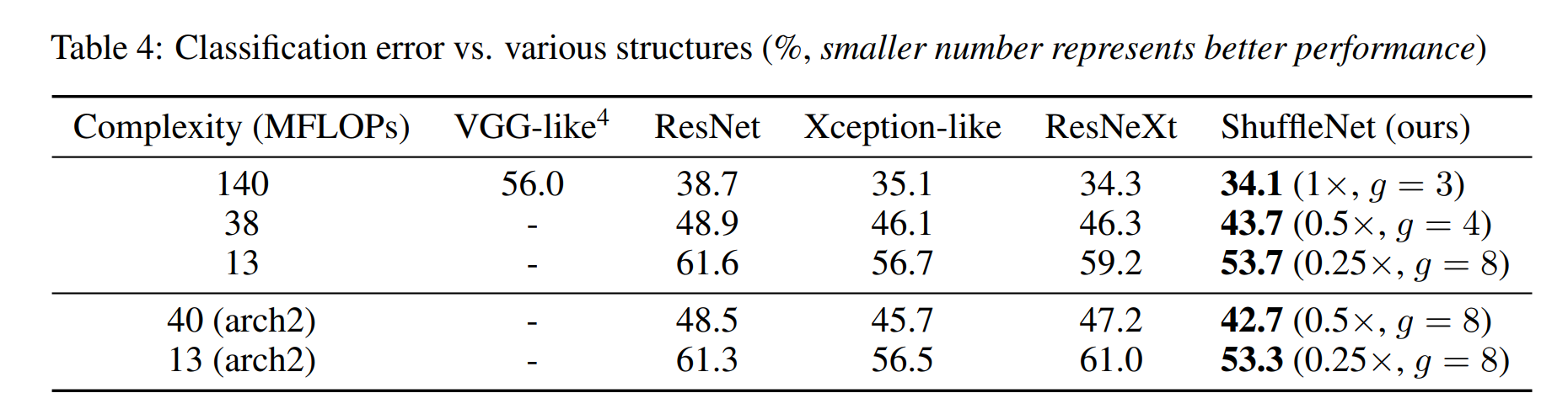
Comparison with Other Structure Units
Recent leading convolutional units in VGG, ResNet, GoogleNet, ResNeXt and Xception have pursued state-of-the-art results with large models (e.g. ≥ 1GFLOPs), but do not fully explore low-complexity conditions.
VGG, ResNet, GoogleNet, ResNeXt 및 Xception는 큰 모델로서 SOTA를 주장했지만(예: γ 1GFLOP), low-complexity conditions을 고려하지 않았다.
In this section we survey a variety of building blocks and make comparisons with ShuffleNet under the same complexity constraint.
이 섹션에서는 다양한 구성 요소를 조사하고 complexity constraint조건에서 ShuffleNet과 비교한다.
For fair comparison, we use the overall network architecture as shown in Table 1.
공정한 비교를 위해 표 1과 같이 전체 네트워크 아키텍처를 사용한다.
We replace the ShuffleNet units in Stage 2-4 with other structures, then adapt the number of channels to ensure the complexity remains unchanged.
ShuffleNet의 2-4 stage를 다른 구조로 교체하고 채널 수를 조정하여 complexity가 변하지 않도록 한다.
The structures we explored include:
조사한 구조는 다음과 같다:
VGG-like. Following the design principle of VGG net, we use a two-layer 3×3
convolutions as the basic building block.
VGG-like. VGG net의 설계에 따라 기본적으로 2개의 3×3 convolution을 사용한다.
we add a Batch Normalization layer after each of the convolutions to make end-to-end training easier.
각 convolutions 후 Batch Normalization layer을 추가하여 end-to-end로 학습을 더 쉽게 만든다.
ResNet. We adopt the "bottleneck" design in our experiment, which has been demonstrated more efficient in. the bottleneck ratio3 is also 1 : 4.
ResNet. 우리는 실험에서 ResNet에서 입증된 "bottleneck" 디자인을 채택한다. 이는 더 효율적임이 입증되었고 bottleneck ratio3 또한 1:4 이다.
Xception-like. The original structure proposed in involves fancy designs or hyperparameters for different stages, which we find difficult for fair comparison on small models.
Xception-like. Xception에서 제안된 구조는 다양한 단계에 대한 여러 디자인에 따른 다양한 hyperparameters를 포함하며, 우리의 모델과 공정하게 비교하기는 어렵다.
Instead, we remove the pointwise group convolutions and channel shuffle operation from
ShuffleNet (also equivalent to ShuffleNet with g = 1).
대신, 우리는 ShuffleNet에서 pointwise group convolutions과 channel shuffle operation을 제거한다. (또한 g = 1인 ShuffleNet과 동일하다).”
The derived structure shares the same idea of "depthwise separable convolution", which is called an Xception-like structure here.
유도된 구조는 'depthwise separable convolution’의 같은 아이디어를 공유하며, 여기서 Xception-like 구조라고 불린다.
ResNeXt. We use the settings of cardinality = 16 and bottleneck ratio = 1 : 2. We also explore other settings, e.g. bottleneck ratio = 1 : 4, and get similar results.
We use exactly the same settings to train these models.
ResNeXt. cardinality = 16과 bottleneck ratio = 1 : 2의 설정을 사용한다. 다른 설정으로는 예를 들어 bottleneck ratio = 1 : 4를 설정하고 비슷한 결과를 얻는다. 이러한 모델을 훈련시키기 위해 완전히 같은 설정을 사용한다.”
ResNeXt는 ResNet의 변형으로, "cardinality"와 "bottleneck ratio"이라는 두 가지 중요한 hyper-parameters를 도입한다. "Cardinality"는 group convolutions에서 그룹의 수를 의미하며, "bottleneck ratio"은 bottleneck 디자인에서 1x1 convolutions layer의 출력 채널 수와 3x3 convolutions layer의 출력 채널 수의 비율을 의미한다. 이 부분에서는 cardinality = 16과 bottleneck ratio = 1 : 2의 설정을 사용하며, 다른 설정을 탐색해도 비슷한 결과를 얻는다고 설명하고 있다. 이는 ResNeXt의 성능이 이러한 hyper-parameters의 특정 값에 크게 의존하지 않음을 의미한다.
We use exactly the same settings to train these models. Results are shown in Table 4.
우리는 이 모델들을 훈련시키기 위해 정확히 같은 설정을 사용한다. 결과는 표 4에 나와 있다.
Our ShuffleNet models outperform most others by a significant margin under different complexities.
우리의 ShuffleNet 모델은 다양한 complexities에서 대부분의 다른 모델보다 훨씬 우수하다.
Interestingly, we find an empirical relationship between feature map channels and classification accuracy.
흥미롭게도, 우리는 특징 지도 채널과 분류 정확도 사이의 경험적 관계를 발견한다.
For example, under the complexity of 38 MFLOPs, output channels of Stage 4 (see Table 1) for VGG-like, ResNet, ResNeXt, Xception-like, ShuffleNet models are 50, 192, 192, 288, 576 respectively, which is consistent with the increase of accuracy.
예를 들어, 38 MFLOPs의 복잡성 하에서, VGG-like, ResNet, ResNeXt, Xception-like, ShuffleNet 모델의 4단계 출력 채널(표 1 참조)은 각각 50, 192, 192, 288, 576이며, 이는 정확도의 증가와 일관성이 있다.(여러 모델 아키텍처의 출력 채널 수와 그들의 정확도 사이의 관계를 설명)
출력 채널 수는 네트워크가 한 번에 처리할 수 있는 특징의 수를 의미한다. 출력 채널 수가 많을수록, 네트워크는 더 많은 특징을 추출하고 더 복잡한 패턴을 학습할 수 있다.
Since the efficient design of ShuffleNet, we can use more channels for a given computation budget, thus usually resulting in better performance.
ShuffleNet의 효율적인 설계 덕분에 주어진 계산 예산에 더 많은 채널을 사용할 수 있으므로 일반적으로 성능이 향상된다.
It can be observed that ShuffleNet still achieves outstanding results over other structures.
ShuffleNet은 여전히 다른 구조에 비해 뛰어난 결과를 달성하고 있음을 알 수 있다.
Note that the above comparisons do not include GoogleNet or Inception series [30, 31, 29]. We find it nontrivial to generate such Inception structures to small networks because the original design of Inception module involves too many hyper-parameters.
성능 비교에서 GoogleNet 또는 Inception series [30, 31, 29]를 포함하지 않는다. 왜냐하면 Inception 모듈의 설계가 너무 많은 hyper-parameters를 포함하기 때문에 우리의 네트워크와의 비교는 맞지 않다.
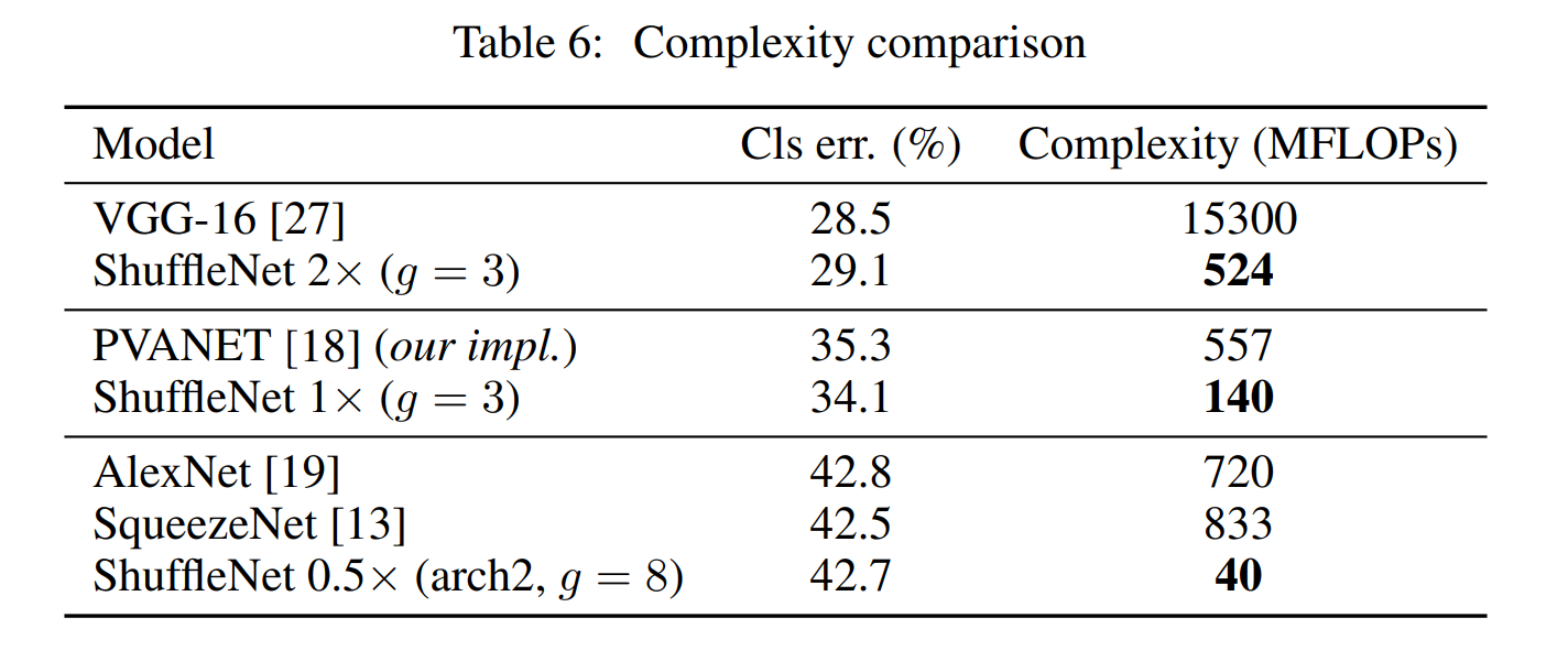
As a reference, Kim et al. have recently proposed a lightweight network structure named PVANET [18] which adopts Inception units.
참고로 Kim 등. 최근에는 Inception 단위를 채택하는 PVANET[18]이라는 이름의 경량 네트워크 구조를 제안했다.
Our reimplemented PVANET (with 224×224 input size) has 35.3% classification error with a computationcomplexity of 557 MFLOPs, while our ShuffleNet 2x model (g = 3) gets 29.1% with 524 MFLOPs (see Table 6). So even though lack of direct comparisons, it is unlikely for Inception to surpass ShuffleNet in trivial settings.
재구현된 PVANET(224×224 입력 크기)은 35.3%의 분류 오류와 557 MFLOPs의 계산 복잡성을 가진 반면 ShuffleNet 2x 모델(g = 3)은 524 MFLOPs로 29.1%를 얻었습니다(표 6 참조). 따라서 직접적인 비교가 부족하더라도 Inception이 사소한 설정에서 ShuffleNet을 능가할 가능성은 낮습니다.
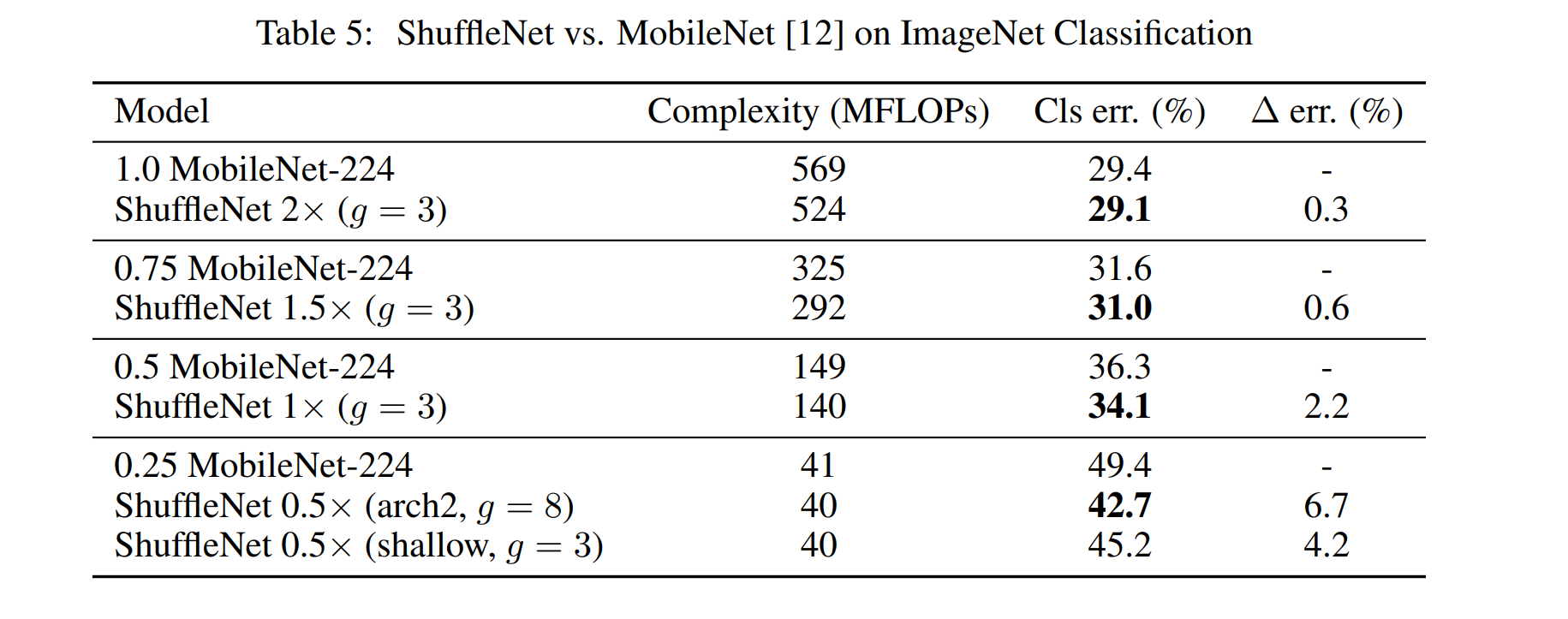
Comparison with MobileNets and Other Frameworks
Recently Howard et al. have proposed MobileNets which mainly focus on efficient network
architecture for mobile devices.
최근 Howard 등 주로 모바일 장치를 위한 효율적인 네트워크에 초점을 맞춘 MobileNets를 제안했다.
MobileNet takes the idea of depthwise separable convolution from and achieves state-of-the-art results on small models.
MobileNet은 depthwise separable convolution의 아이디어를 가지고 small models에서 SOTA를 달성한다.
Table 5 compares classification scores under a variety of complexity levels.
표 5는 다양한 complexity levels에서 classification scores를 비교한다.
It is clear that our ShuffleNet models are superior to MobileNet for all the complexities.
ShuffleNet 모델이 모든 복잡성에서 MobileNet보다 우수하다는 것은 분명하다.
Though our ShuffleNet network is specially designed for small models (< 150 MFLOPs), we find it is still slightly better than MobileNet for higher computation cost.
ShuffleNet네트워크는 small models(<150 MFLOP)을 위해 특별히 설계되지만 여전히 더 높은 computation cost에 대해서도 MobileNet보다 성능이 약간 좋다는 것을 발견했다.
For smaller networks (~40 MFLOPs) ShuffleNet surpasses MobileNet by 6.7%.
소규모 네트워크(~40 MFLOP)의 경우 ShuffleNet이 MobileNet을 6.7% 능가한.
Note that our ShuffleNet architecture contains 50 layers (or 44 layers forarch2) while MobileNet only has 28 layers.
ShuffleNet 아키텍처에는 50개의 레이어(arch2의 경우 44개의 레이어)가 포함된 반면 MobileNet은 28개의 레이어만 포함되어 있다.
For better understanding, we also try ShuffleNet on a 26-layer architecture by removing half of the blocks in Stage 2-4 (see "ShuffleNet 0.5× shallow(g = 3)" in Table 5).
더 잘 이해하기 위해 2-4 Stage에서 블록의 절반을 제거하여 26-layer 아키텍처의 ShuffleNet을 사용해 본다.(표 5의 "ShuffleNet 0.5×half(g = 3)" 참조).
Results show that the shallower model is still significantly better than the corresponding MobileNet, which implies that the effectiveness of ShuffleNet mainly results from its efficient structure, not the depth.
결과는 hallower model이 MobileNet보다 여전히 낫다는 것을 보여주는데, 이는 ShuffleNet의 효과가 깊이가 아닌 효율적인 구조에서 주로 비롯된다는 것을 의미한다.
Generalization Ability
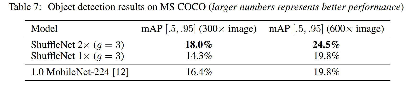
To evaluate the generalization ability for transfer learning, we test our ShuffleNet model on the task of MS COCO object detection.
transfer learning의 일반화 능력을 평가하기 위해 작업에서 COCO object detection으로 ShuffleNet 모델을 테스트한다.
We adopt Faster-RCNN as the detection framework and use the publicly released Caffe code for training with default settings.
Faster-RCNN을 detection 프레임워크로 사용하고 기본설정으로 공개된 코드를 가지고 training에 사용한다.
the models are trained on the COCO train+val dataset excluding 5000 minival images and we conduct testing on the minival set. Table 7 shows the comparison of results trained and evaluated on two input resolutions.
모델은 5000개의 minival 이미지를 제외한 COCO train+val 데이터 세트에서 훈련되며 minival set에서 테스트를 수행한다.
표 7은 두 개의 입력 해상도에 따라 훈련되어진 결과를 보여준다.
Comparing ShuffleNet 2× with MobileNet whose complexity are comparable (524 vs. 569 MFLOPs), our ShuffleNet 2× surpasses MobileNet by a significant margin on both resolutions;
복잡성이 비슷한 ShuffleNet 2×와 MobileNet (524 vs. 569 MFLOPs)을 비교할 때, ShuffleNet 2×는 두 가지 해상도 비교에서 MobileNet을 큰 차이로 앞선다;
our ShuffleNet 1× achieves comparable results with MobileNet on 600× resolution, but has ~4× complexity reduction.
우리의 ShuffleNet 1×는 600× 해상도에서 MobileNet과 유사한 결과를 달성하지만, 복잡성은 약 4배 감소한다.
We conjecture that this significant gain is partly due to ShuffleNet’s simple design of architecture without bells and whistles.
이런 큰 향상이 ShuffleNet의 복잡한 기능 없는 간단한 아키텍처 디자인 때문이라고 추측한다.
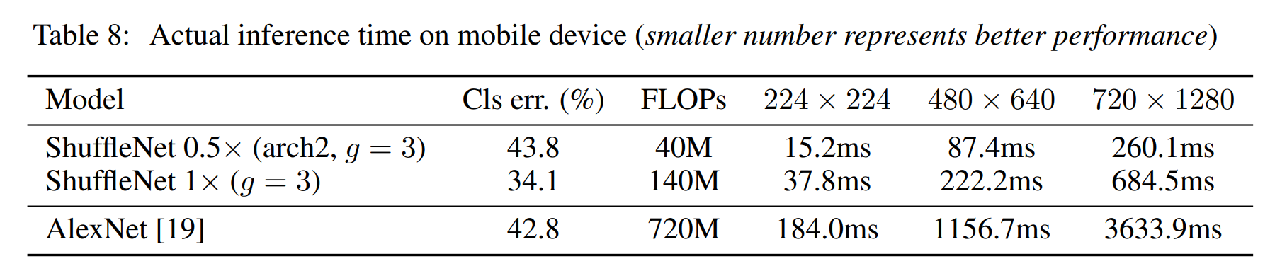
Actual Speedup Evaluation
Finally, we evaluate the actual inference speed of ShuffleNet models on a mobile device with an
ARM platform.
마지막으로, 우리는 ARM 아키텍처 모바일 장치에서 ShuffleNet 모델의 실제 추론 속도를 평가한다.
As shown in Table 8, three input resolutions are exploited for the test.
표 8에 나타난 바와 같이, 세 가지 입력 해상도가 테스트에 활용된다.
Due to memory access and other overheads, we find every 4× theoretical complexity reduction usually results in ~2.6× actual speedup in our implementation.
메모리 접근 및 기타 오버헤드로 인해, theoretical complexity 감소는 4배이나, 실제로는 약 2.6배의 속도 향상을 얻는다는 것을 발견했.
Nevertheless, compared with AlexNet our ShuffleNet 0.5× model still achieves ~13× actual speedup under comparable classification accuracy (the theoretical speedup is 18×), which is much faster than previous AlexNet-level models or speedup approaches.
그럼에도 불구하고, AlexNet과 비교할 때, 우리의 ShuffleNet 0.5× 모델은 비슷한 classification accuracy에서 약 13배의 실제 속도 향상을 달성한다.(이론적 속도 향상은 18배입니다), 이는 이전의 AlexNet 수준의 모델이나 속도 향상 방법보다 훨씬 빠르다. (이론적으로는 18배의 속도 향상을 예상했지만, 실제 구현에서는 약 13배의 속도 향상만을 달성했다는 것)

Comment