ResNet 논문리뷰

서론

Kaiming He, Xiangyu Zhang, Shaoqing Ren, Jian Sun; "Deep Residual Learning for Image Recognition", Proceedings of the IEEE Conference on Computer Vision and Pattern Recognition (CVPR), 2016, pp. 770-778, Deep Residual Learning for Image Recognition
이 논문은 2015년에 공개되었으며, ResNet은 신경망이 깊어질수록 발생하는 Gradient Vanishing문제를 해결하기 위해 residual learning이라는 개념을 도입함으로써 해결하였다.
ResNet 모델은 ILSVRC (ImageNet Large Scale Visual Recognition Challenge) 2015 분류 및 검출 부문에서 1위를 차지했다.

Abstact

We present a residual learning framework to ease the training of networks that are substantially deeper than those used previously.

이전에 사용된 것보다 훨씬 더 깊은 네트워크의 훈련을 용이하게 하기 위해 residual learning(잔여 학습) framework를 제시한다.

On the ImageNet dataset we evaluate residual nets with a depth of up to 152 layers 8 times deeper than VGG nets but still having lower complexity.

ImageNet dataset으로 VGG 보다 8배 깊은 152 layer를 사용했음에도 여전히 복잡도가 높지 않다.

An ensemble of these residual nets achieves 3.57% error on the ImageNet test set.

ImageNet dataset에서 3.5%의 error rate를 달성했다.

Introduction

Research background

Deep convolutional neural networks have led to a series of breakthroughs for image classification.
Deep convolutional neural Network는 이미지 분류 분야에서 획기적인 발전을 이끌었다.

Recent Research

Recent evidence reveals that network depth is of crucial importance, and the leading results on the challenging ImageNet dataset all exploit “very deep”models, with a depth of sixteen to thirty.
최근의 연구는 네트워크 깊이가 매우 중요하다는 것을 보여주며, ImageNet dataset에 대해 좋은 결과가 나온 모델들은 모두 16-30의 깊이로 "매우 깊은" 모델을 활용한다.
Driven by the significance of depth, a question arises: Is learning better networks as easy as stacking more layers?
그래서 “depth를 늘리는 것만으로 쉽게 성능을 향상 시킬 수 있을까?”라는 의문을 갖는데 여기서 두 가지 문제가 발생한다.

Convergence Problem

An obstacle to answering this question was the notorious problem of vanishing/exploding gradients, which hamper convergence from the beginning.
gradient vanishing/exploding 발생되며 모델의 학습 초기부터 잘 학습(수렴)되지 못하도록 방해한다.
This problem, however, has been largely addressed by normalized initialization and intermediate normalization layers, which enable networks with tens of layers to start converging for stochastic gradient descent (SGD) with backpropagation.
normalized initialization, intermediate normalization layers를 통해 크게 개선되어 Back propagation와 SGD로 수십개의 layer를 가진 네트워크가 수렴해 나가도록 하면서 이 문제를 해결한다.

Degradation Problem

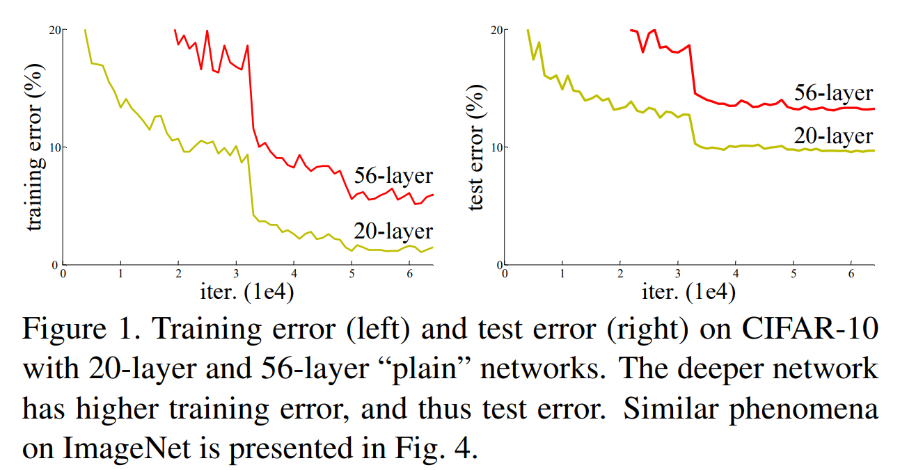
When deeper networks are able to start converging, a degradation problem has been exposed: with the network depth increasing, accuracy gets saturated (which might be unsurprising) and then degrades rapidly.
네트워크가 학습할 때 네트워크의 깊이가 증가함에 따라 accuracy가 saturate되고 그 이후로degradation(성능 저하)문제가 빠르게 나타난다.
Unexpectedly, such degradation is not caused by overfitting, and adding more layers to a suitably deep model leads to higher training error, as reported in and thoroughly verified by our experiments.
이러한 degradation 문제는 overfitting이 원인이 아니라, Model의 depth가 깊어짐에 따라 training-error가 높아진다는 것이다.
아래 그림은 신경망이 깊어지는 경우 어떤 결과가 나오는지 CIFAR-10 학습 데이터로 20-layer와 56-layer에 대해 비교 실험했다.

Summary

이론적으로는 레이어가 깊어질수록 고차원의 feature 들을 학습해 낼 수 있어서 classification 성능이 높아진다는 것이 알려져 있지만 일정 레이어 이상으로 깊이가 깊어지면 성능이 나빠지게 되어(gradient Vanishing나 overfitting 문제) 레이어의 수를 제한적으로 사용해 왔다.
그것의 예로 위 왼쪽 그래프를 보면 34 레이어가 오히려 18 레이어 보다 성능이 나빠진 실험 결과를 볼 수 있다.

Propose

Let us consider a shallower architecture and its deeper counterpart that adds more layers onto it.
더 적은 수의 계층을 가진 '얕은'(shallower) 신경망과 그보다 더 많은 계층을 추가하여 '깊게'(deeper) 만든 신경망을 비교하자는 제안이다.
There exists a solution by construction to the deeper model: the added layers are identity mapping, and the other layers are copied from the learned shallower model.
깊은 모델은 shallow모델에 추가한 layer들은 identity mapping(입력이 그대로 출력으로 나오는 함수)으로 돼있고 나머지 layer는 이미 학습된 shallower model에서 복사된 것이다.
The existence of this constructed solution indicates that a deeper model should produce no higher training error than its shallower counterpart. But experiments show that our current solvers on hand are unable to find solutions that are comparably good or better than the constructed solution
이렇게 구성된 해결책은 깊은 모델이 얕은 모델보다 더 traning error가 더 낮아야 한다.
추측으론 깊은 신경망의 추가 계층들은 identity mapping을 통해 얕은 신경망의 성능을 그대로 유지하면서 더 깊이 layer를 쌓았음으로 성능이 더 좋거나 최소한 나쁘지 않아야 한다는 것 같다.
그러나 이는 좋은 해결책이 아니라는 결과를 얻었다.
In this paper, we address the degradation problem by introducing a deep residual learning framework.
이 논문에서는 degradation problem를 해결하기 위해 deep residual leraning framework를 제안한다.
Instead of hoping each few stacked layers directly fit a desired underlying mapping, we explicitly let these layers fit a residual mapping
쌓여진 레이어가 그 다음 레이어에 바로 적합되는 것이 아니라 Residual mapping에 적합하도록 만들었다.

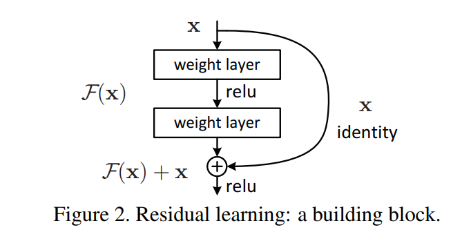
"Formally, denoting the desired underlying mapping as H(x), we let the stacked nonlinear layers fit another mapping of F(x) := H(x)−x. The original mapping is recast into F(x)+x."
Original Mapping(기존의 학습방식)에서는 그냥 \(H(X)\)를 예측하는 것이다. 논문에서는 \(F(X) =H(X) -X\)라는 Residual Mapping을 제안한다.
- 입력 x에 대한 출력을 \(H(X)\)라 하면 입력과 출력의 변화량(잔차=Residual)을 \(F(X)\)로 표현하면 \(F(X) = H(X) - X\)라고 생각 할 수 있다. 이 \(F(X)\)를 예측하는 것이 Residual Mapping이다.
We hypothesize that it is easier to optimize the residual mapping than to optimize the original, unreferenced mapping.
Residual mapping이 기존의 Original mapping보다 optimize하기 쉽다는 것을 가정한다.
To the extreme, if an identity mapping were optimal, it would be easier to push the residual to zero than to fit an identity mapping by a stack of nonlinear layers.
극단적으로 identity mapping이 최적이라고 할 때, 비선형 레이어를 쌓아서 identity mapping을 맞추는 것 보다 잔차를 0으로 만드는 것이 더 쉽습니다.
- H(x)를 단순히 맞추는 것보다 변화량(잔차=Residual) F(x)를 0으로 수렴하게 만드는 것이 더 쉽기 때문이다. \(0 = H(X) - X = H(X) = X\)
The formulation of F(x) +x can be realized by feedforward neural networks with “shortcut connections” (Fig. 2). Shortcut connections are those skipping one or more layers.
F(x) + x는 Shortcut Connection과 동일하다. 이는 하나 또는 이상의 layer를 skip하게 만들어준다이 모델의 아키텍처를 보면 건너뛴다는 것을 볼 수 있다.
In our case, the shortcut connections simply perform identity mapping, and their outputs are added to the outputs of the stacked layers (Fig. 2). Identity shortcut connections add neither extra parameter nor computational complexity.
shortcut connection은 단순히 identity mapping을 수행하며, 결과는 stacked layer에서 나온 출력과 shortcut connetcion이 더해집니다 (Fig. 2). Identity shortcut connections은 추가적인 parameter나 computational complexity 요구하지 않는다.
The entire network can still be trained end-to-end by SGD with backpropagation, and can be easily implemented using common libraries (e.g., Caffe [19]) without modifying the solvers.
또한 전체 네트워크는 역전파와 함께 SGD에 의해 end-to-end로 학습되고, 기존 라이브러리를 이용하여 간단히 구현 가능하다.
Our 152 layer residual net is the deepest network ever presented on ImageNet, while still having lower complexity than VGG nets. Our ensemble has 3.57% top-5 error on the ImageNet test set, and won the 1st place in the ILSVRC 2015 classification competition.
152 layer residual net을 사용하여 VGGNet보다 낮은 복잡도로 top-5 error rate가 3.57%로 놀라운 성능을 얻었으며 ILSVRC 2015 classification에서 1위를 차지했다.

Summary

입력 x에 대한 출력을 H(x)라 하고 입력과 출력의 변화량을 F(x)로 표현하면 F(x) = H(x) - x 라고 생각 할 수 있다.
다. 왜냐하면 최종 출력H(x)이고 입력 x의 차가 변화량(잔차=Residual)이기 때문이다. 따라서 F(x)를 예측하는 것이 Residual Mapping이다.
그러면 최종 출력은 H(x) = F(x) + x 로 계산될 수 있다. 수식을 해석해보면 변화량 F(x)를 예측하고 이 변화량 F(x)에 입력 x에 더함으로써 최종 출력 H(x)를 얻는 방식이다.
이 논문에서는 입력 x에 대해 변화량 F(x)를 예측하는 Residual Mapping이 기존의 identity mapping보다 최적화하기 쉽다는 것을 주장한다.
왜냐하면 변화량(잔차=Residual) F(x)를 0에 가까이 만드는 것이 비선형 레이어를 쌓아서 만든 복잡한 함수 H(x)를 직접 맞추는 것보다 더 쉽기 때문이다.
이러한 이유로, 이 논문은 'Residual Learning'이라는 새로운 학습 방식을 제안하고 있습니다.
실제로 Residual 구조로 인하여 위 실험과 같이 layer의 깊이가 깊어짐에 따라서 모델의 성능이 더 좋아진 것을 확인할 수 있다.
즉 plain 한 모델의 경우에는 layer가 일정 깊이 이상으로 깊어지면 학습이 안되었지만 Residual 구조에서는 layer가 깊어져도 학습이 잘 되는 것을 확인할 수 있다.
기존의 layer가 깊어질수록 발생하는 gradient Vanishing문제를 개선할 수 있는 path가 생겼고 따라서 입력의 작은 변화도 깊은 layer에서 알아챌 수 있도록 한다는 것이었고 실제 실험의 결과로 나타난다. (Experiments 확인)

Related Work

Residual Representation

In image recognition, VLAD is a representation that encodes by the residual vectors with respect to a dictionary, and Fisher Vector can be formulated as a probabilistic version of VLAD
Image Recognition에서 VLAD는 Residual Vector를 이용하여 Encoding 하는 방법이다. Fisher Vector는 VLAD의 확률론적 버전이다.
Both of them are powerful shallow representations for image retrieval and classification
VLAD와 Fisher Vector는 이미지 검색(Image Retrieval과 classification)에서 강력한 얕은(shallow) 표현 방법이다.
For vector quantization, encoding residual vectors is shown to be more effective than encoding original vectors.
original vector를 encoding하는 것보다 residual vector를 인코딩하는 것이 vector quantization에 더 효과적이다.
These methods suggest that a good reformulation or preconditioning can simplify the optimization.
따라서 original vector가 아닌 Residual vector를 이용함으로써 단순한 형태로 재구성(reformulation)하거나 적절한 사전조건(preconditioning )을 설정하여 최적화 문제를 더 쉽게 해결할 수 있음을 나타낸다.

VLAD & Fisher Vector

VLAD(Vector of Locally Aggregated Descriptors), Fisher Vector는 전통적인 컴퓨터 비전 알고리즘 중 하나로, 이미지의 특징을 벡터로 표현하는 방법
VLAD
- VLAD는 k-means clustering을 사용하여 이미지의 local한 feature(색상, 질감, 모양 등)을 clustering한다. 각 local feature에 대해, 이 feature가 가장 가까운 cluster의 중심과 얼마나 다른지를 계산하는데 이 차이를 모든 로컬 특징에 대해 누적하고, 이를 고차원의 벡터로 인코딩하여 VLAD를 생성한다. VLAD는 각 클러스터에 대한 특징의 편차를 집계함으로써, 이미지의 특징을 간결하게 요약한다.
Fisher Vector
- Gaussian Mixture Model(GMM)을 사용하여 이미지의 local한 feature들을 Gaussian Mixture Model(GMM)'라는 통계적인 방법을 통해 “특징 분포”를 만든다. 그리고 각 local feature에 대해, 이 특징이 GMM의 각 구성 요소에 얼마나 기여하는지 측정한다.
- 이렇게 하면 각 featur가 이미지 전체에서 어떤 역할을 하는지 알 수 있는데 이 정보를 모아서 벡터를 만드는데 이 벡터가 Fisher Vector이다.

Short Connections

Concurrent with our work, “highway networks” present shortcut connections with gating functions.
highway networks는 shortcut connections에 parameter를 가진 gating function이 존재한다.
These gates are data-dependent and have parameters, in contrast to our identity shortcuts that are parameter-free.
이 gate는 paramter에 대해서 의존적인데 우리가 사용하는 short connection은 parameter가 없다.
When a gated shortcut is “closed” (approaching zero), the layers in highway networks represent non-residual functions.
gate의 paramter가 닫히게 되면(0에 가까워지면) Residual function인 F(x)(앞서 설명한 변화량을 타나태는 값)를 표현하지 못한다.
On the contrary, our formulation always learns residual functions; our identity shortcuts are never closed, and all information is always passed through, with additional residual functions to be learned.
이 논문에서 사용하는 residual function은 결코 닫힐 일이 없으며 input에 대한 모든 정보들은 통과하고 변화량(Residual Function)F(x)이 잘 학습될 수 있다.
In addition, high way networks have not demonstrated accuracy gains with extremely increased depth (e.g., over 100 layers).
또한, high way networks는 극도로 깊어진 네트워크(예: 100층 이상)에서 정확도 향상을 보여주지 못했다.
따라서 논문에서 제시하는 short connetion이 효과적이다를 설명하고 있다.

Deep Residual Learning

3.1 Residual learning

이러한 이유로, 이 논문은 'Residual Learning'이라는 새로운 학습 방식을 제안하고 있습니다.

3.2 Identity Mapping by Shortcuts

We adopt residual learning to every few stacked layers.
모든 few stacked layer마다 residual mapping을 적용했다.

y = F(x, \; \{ W_i \})+x

The function F(x, {Wi}) represents the residual mapping to be learned.
F(x, {Wi}) 는 학습될 residual mapping을 의미한다.

F(x, \{W_i\})

F = W2σ(W1x) in which σ denotes ReLU and the biases are omitted for simplifying notations.
F = W2σ(W1 x) 에서 σ는 ReLu를 의미한다.

F = W_2\sigma(W_1x)

The operation F + x is performed by a shortcut connection and element-wise addition
F + x 연산이 shortcut connection을 의미하고 element-wise addition이다.
The shortcut connections in Eqn.(1) introduce neither extra parameter nor computation complexity.
앞서 소개한 shortcut connetions는 parameter도 없고 computation complexity도 없다.
The dimensions of x and F must be equal.
위 수식에서는 x와 F의 차원이 같아야한다.
If this is not the case (e.g., when changing the input/output channels), we can perform a linear projection Ws by the shortcut connections to match the dimensions
만약 F(x, \{W_i\}) 수식의 x와 F의 차원이 다를 경우 linear projection인 Ws를 통해 short connection의 차원을 맞춰준다.

y = F(x, \{W_i\}) +W_sx

3.3 Network Architectures

We have tested various plain/residual nets, and have observed consistent phenomena.
Plain Network과 Residual Network 두 네트워크를 가지고 실험했다.
Plain Network
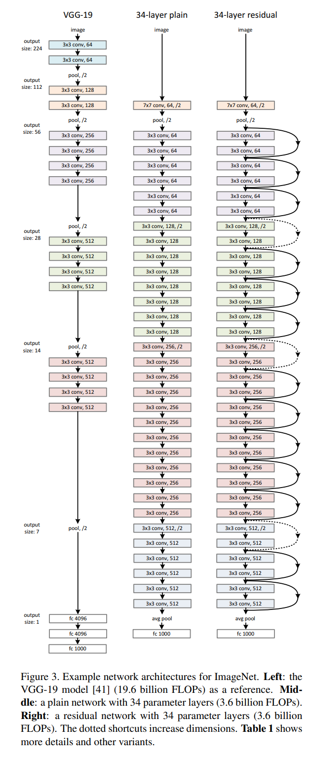
- Our plain baselines (Fig. 3, middle) are mainly inspired by the philosophy of VGG nets.
- VGG net 철학에 영감을 받았다.
Residual Network
- Based on the above plain network, we insert shortcut connections (Fig. 3, right) which turn the network into its counterpart residual version.
- 위의 plain network에 shortcut connection을 삽입했다.
- The identity shortcuts (Eqn.(1)) can be directly used when the input and output are of the same dimensions (solid line shortcuts in Fig. 3).
- input과 output의 차원이 같은 경우 위 수식을 사용하면 된다.(그림에서는 실선으로 표기)
- The projection shortcut in Eqn.(2) is used to match dimensions (done by 1×1 convolutions).
- When the dimensions increase (dotted line shortcuts in Fig. 3), we consider two options: (A) The shortcut still performs identity mapping, with extra zero entries padded for increasing dimensions. This option introduces no extra parameter;
- 차원이 다른경우 두가지 옵션이 있는데 첫번째는 zero padding을 추가해 차원을 맞춰주는 경우가 있다 이때 추가적인 parameter가 필요없다. (그림에서 점선으로 표기)
- The projection shortcut in Eqn.(2) is used to match dimensions (done by 1×1 convolutions).
- 차원을 맞춰주기 위해 projection layer인 1x1convolution을 사용한다.

3.4 Implementation

A 224×224 crop is randomly sampled from an image or its horizontal flip, with the per-pixel mean subtracted.
이미지 전체 픽셀에 대한 평균값을 각 픽셀에서 전부 빼고 horizontal flip된 이미지로부터 224x224 Image
The standard color augmentation in is used.
standard color augmentation이 사용된다.
We adopt batch normalization (BN) right after each convolution and before activation
각 convolution이후와 activiation전에 Batch Normalization을 적용한다.
We use SGD with a mini-batch size of 256.
256의 미니배치를 사용한다.
The learning rate starts from 0.1 and is divided by 10 when the error plateaus, and the models are trained for up to 60 × 10^4 iterations.
학습률은 0.1 부터 시작하며 에러가 안정되면 lr에 0.1씩 곱해준다. 그리고 iteration은 60만번 까지 한다.
We use a weight decay of 0.0001 and a momentum of 0.9.
0.0001의 weight decay와 0.9의 momentum 사용한다.
We do not use dropout.
Dropout을 사용하지 않았다.

Experiments

ImageNet Classification

We evaluate our method on the ImageNet 2012 classification dataset [36] that consists of 1000 classes.
1000개의 클래스로 구성된 ImageNet 2012 dataset을 사용했다.

Plain Networks

We first evaluate 18-layer and 34-layer plain nets. The results in Table 2 show that the deeper 34-layer plain net has higher validation error than the shallower 18-layer plain net.
pain net으로 쌓은 18-layer와 34-layer를 비교하면 34-layer에서 Train error, Test eroor 모두 높은 gradation problem 볼 수 있다.
직관적이지 않은 결과인데, 왜냐하면 일반적으로 신경망이 더 깊어질수록 더 복잡한 패턴을 학습할 수 있으므로 성능이 향상되어야 하기 때문이다.

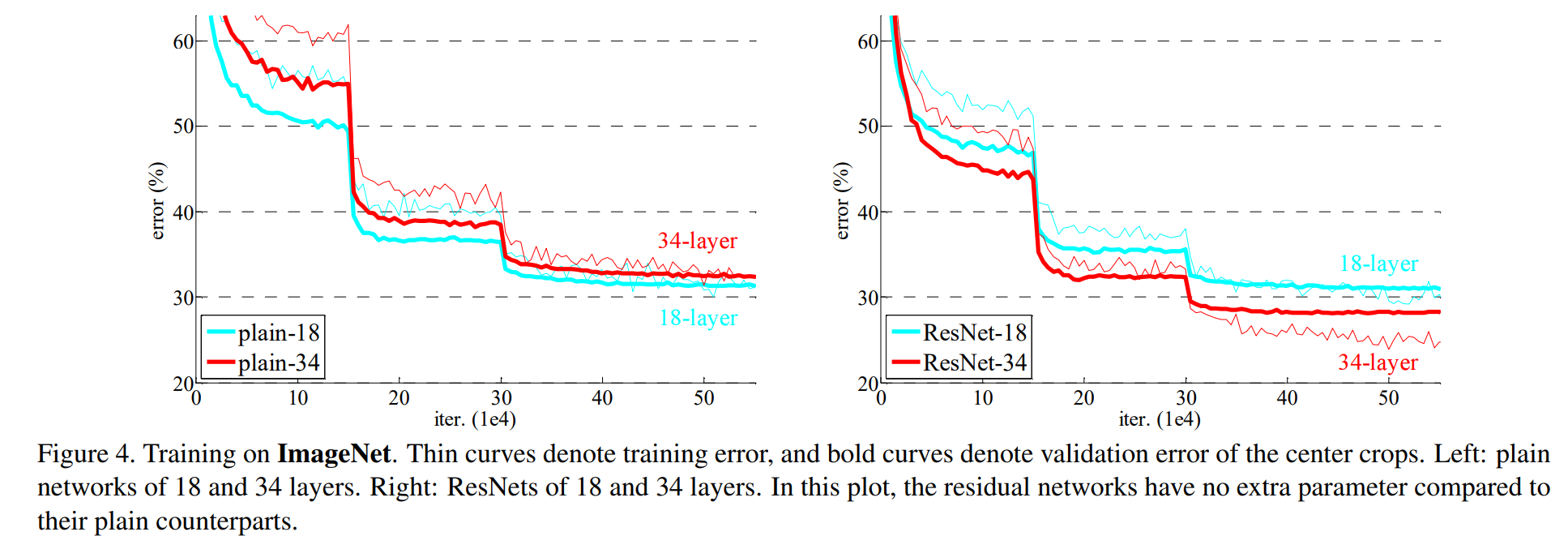
We have observed the degradation problem - the 34-layer plain net has higher training error throughout the whole training procedure, even though the solution space of the 18-layer plain network is a subspace of that of the 34-layer one.
앞서 언급했던 degradation problem의 관점에서 봤을 때 더 깊은 layer모델이 train error가 더 높을 수 있다.
We argue that this optimization difficulty is unlikely to be caused by vanishing gradients.
그러나 최적화가 어려운 것이 gradient vanishing때문이 아닌 것을 알 수 있다.
These plain networks are trained with BN, which ensures forward propagated signals to have non-zero variances. We also verify that the backward propagated gradients exhibit healthy norms with BN.
이 plain networks는 순전파(forward propagated signal)가 0이 되지 않도록 보장하는 배치 정규화(BN)를 사용했고 BN으로 healthy norm을 보여주는 backward propagated gradient를 증명했다.
So neither forward nor backward signals vanish.
따라서 forward, backward signal vanish의 문제가 아니다
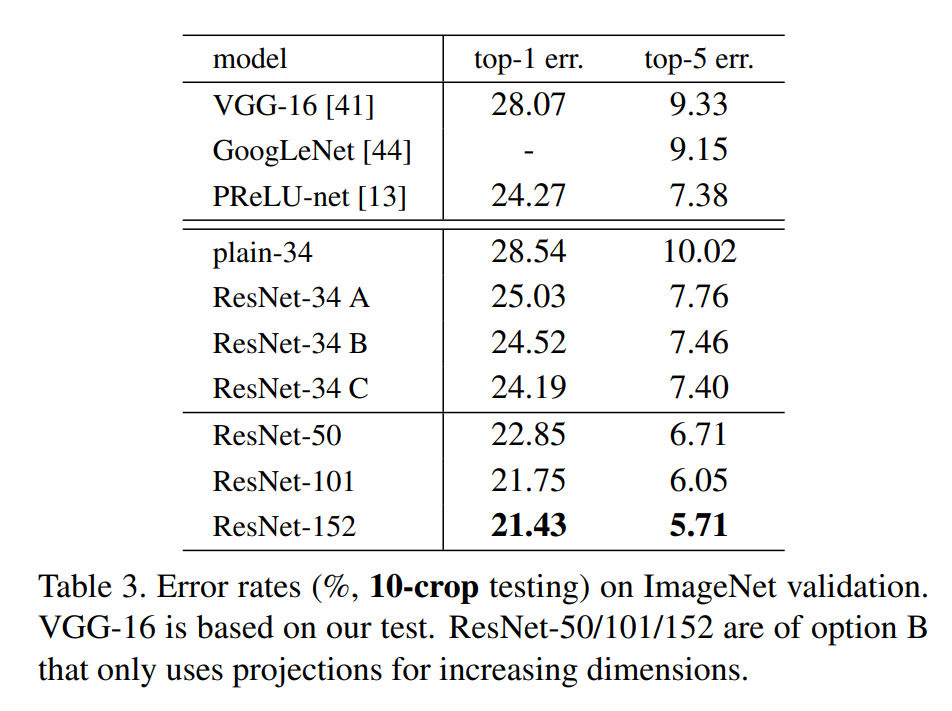
In fact, the 34-layer plain net is still able to achieve competitive accuracy (Table 3), suggesting that the solver works to some extent.
실제로 34layer plain net은 여전히 경쟁력 있는 정확도를 달성할 수 있으며(표 3) solver가 어느 정도 작동함을 볼 수 있다.
We conjecture that the deep plain nets may have exponentially low convergence rates, which impact the reducing of the training error.
training error가 줄어드는데 영향을 주는 low convergence rates가 기하 급수적이기 때문이라고 추측한다.
The reason for such optimization difficulties will be studied in the future.
이런 최적화의 어려움들은 미래에의 연구에 남겨둔다.

Residual Networks

Next we evaluate 18-layer and 34-layer residual nets (ResNets).
18-layer, 34-layer residual network를 평가했다.
we use identity mapping for all shortcuts and zero-padding for increasing dimensions (option A).
모든 shortcuts에서는 identity mapping을 사용했고, 차원을 증가하기 위해 zero-padding을 사용했다. (Option a)
First, the situation is reversed with residual learning the 34-layer ResNet is better than the 18-layer ResNet(by 2.8%).
18-layer ResNet 보다 34-layer ResNet이 성능이 좋다.
This indicates that the degradation problem is well addressed in this setting and we manage to obtain accuracy gains from increased depth.
Second, compared to its plain counterpart, the 34-layer ResNet reduces the top-1 error by 3.5% , resulting from the successfully reduced training error.
plain과 비교했을 때 34-layer ResNet이 성공적으로 training error를 줄였다.
Last, we also note that the 18-layer plain/residual nets are comparably accurate, but the 18-layer ResNet converges faster.
plain/residual nets에서 18-layer들 끼리 비교했을 때 accruracy는 비슷했지만 18-layer ResNet이 더 수렴이 빨랐다. (converges faster)
When the net is “not overly deep” (18 layers here), the current SGD solver is still able to find good solutions to the plain net.
ResNet이 SGD를 사용한 optimization이 더 쉬움을 알 수 있다.

Identity vs. Projection Shortcuts

We have shown that parameter-free, identity shortcuts help with training.
training에서 identity shortcuts을 돕기 위해서 parameter-free 방법을 사용하는데 projection shortcut과 비교해보겠다.
we compare three options: (A) zero-padding shortcuts are used for increasing dimensions, and all shortcuts are parameterfree. (B) projection shortcuts are used for increasing dimensions, and other shortcuts are identity; and (C) all shortcuts are projections.
A. 차원 증가를 위해 zero-padding을 사용하는 경우 (추가 파라미터 없음) B. 차원 증가를 위해 projection shortcuts을 사용, (Ws) (다른 shortcuts은 identity) C. 모든 shortcut들이 projection인 경우
Table 3 shows that all three options are considerably better than the plain counterpart.
B is slightly better than A. We argue that this is because the zero-padded dimensions in A indeed have no residual learning.
B가 A보다 더 나은걸 볼 수 있는데 A는 residual learning이 이뤄지지 않기 때문이다.
C is marginally better than B, and we attribute this to the extra parameters introduced by many (thirteen) projection shortcuts.
C가 B보다 좋은 이유는 projection layer에서 사용된 extra paraemter 때문이다.
(즉 C 제일 좋고 그 다음 B 그 다음 )
But the small differences among A/B/C indicate that projection shortcuts are not essential for addressing the degradation problem.
하지만 projection shortcut에 대한 A, B, C 들 사이의 차이는 degradation 문제를 설명하는데 주요 문제가 아니다.
So we do not use option C in the rest of this paper, to reduce memory/time complexity and model sizes.
C가 성능이 제일 좋았지만 model 이 복잡해지는 것을 위해서 이 논문에서는 사용하지 않겠다.
Identity shortcuts are particularly important for not increasing the complexity of the bottleneck architectures that are introduced below.
identitiy shortcut은 bottleneck architectures의 복잡성을 줄이는데 부분에서 중요하다.(아래 추가설명)

Deeper Bottleneck Architectures

we concerns on the training time that we can afford, we modify the building block as a bottleneck design.
Train시간을 생각해서 아키텍처의 구조를 Bottleneck design을 사용한다.
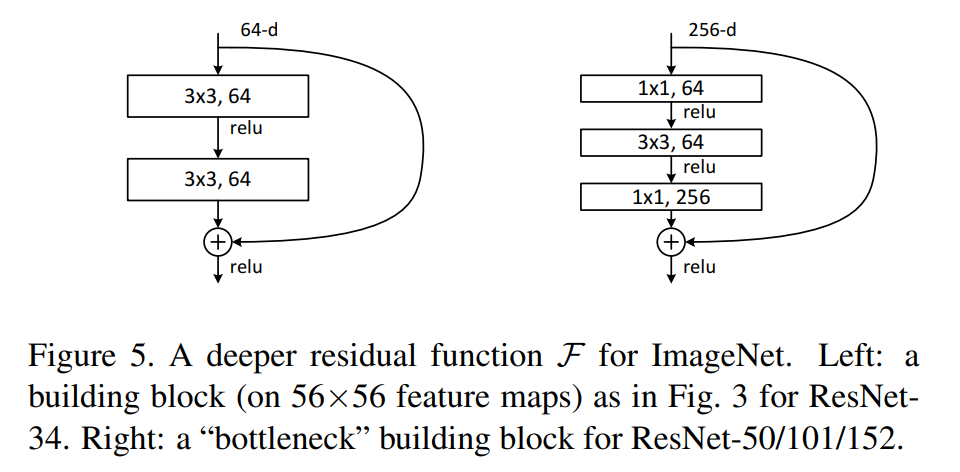
For each residual function F, we use a stack of 3 layers instead of 2 (Fig. 5).
각각 Residual function F를 사용하는데 3층을 쌓을 때, (1 x 1) -> (3 x 3) -> (1 x 1) 순서로 쌓는다.
The three layers are 1×1, 3×3, and 1×1 convolutions, where the 1×1 layers are responsible for reducing and then increasing (restoring) dimensions, leaving the 3×3 layer a bottleneck with smaller input/output dimensions. Fig. 5 shows an example, where both designs have similar time complexity.
1×1 conv는 차원을 줄이는 역할을 하고 3x3 conv는 1x1conv로 부터 입력 차원 줄어든 상태에서복잡한 특징을 학습하는 역할을 한다. 처음 input으로 들어온 차원과 맞춰주기 위해 1x1 conv차원을 원래대로 복원하는 역할을 한다.
이는 기존 구조(Fig5에서의 왼쪽 그림)와 비슷한 복잡성을 가지면서 input과 output의 dimension을 줄이기 때문에 계산 복잡도를 줄일 수 있다.

50-layer ResNet

We replace each 2-layer block in the 34-layer net with this 3-layer bottleneck block, resulting in a 50-layer ResNet. We use option B for increasing dimensions. This model has 3.8 billion FLOPs.
기존에 만들었던 34-layer에 3-layer bottleneck block을 추가해서 50-layer ResNet을 만든다. option B를 사용한다. 연산은 3.8billion FLOPs이다.

101-layer and 152-layer ResNets

We construct 101-layer and 152-layer ResNets by using more 3-layer blocks. Remarkably, although the depth is significantly increased, the 152-layer ResNet (11.3 billion FLOPs) still has lower complexity than VGG-16/19 nets (15.3/19.6 billion FLOPs).
더 많은 3-layer를 추가해서 101-layer와 152-layer를 만든다. 놀랍게도 네트워크의 깊이가 현저히 증가했음에도 152-layer ResNet이 VGG-16/19보다 여전히 작은 복잡성과 적은 연산을 가진다.
The 50/101/152-layer ResNets are more accurate than the 34-layer ones by considerable margins.
또한 50/101/151 layer는 34-layer보다 확실히 더 정확하다.
We do not observe the degradation problem and thus enjoy significant accuracy gains from considerably increased depth.
degradation problem이 발생하지 않으며 깊이의 이점을 살려 성능이 향상됐다.

Comparisons with State-of-the-art Methods

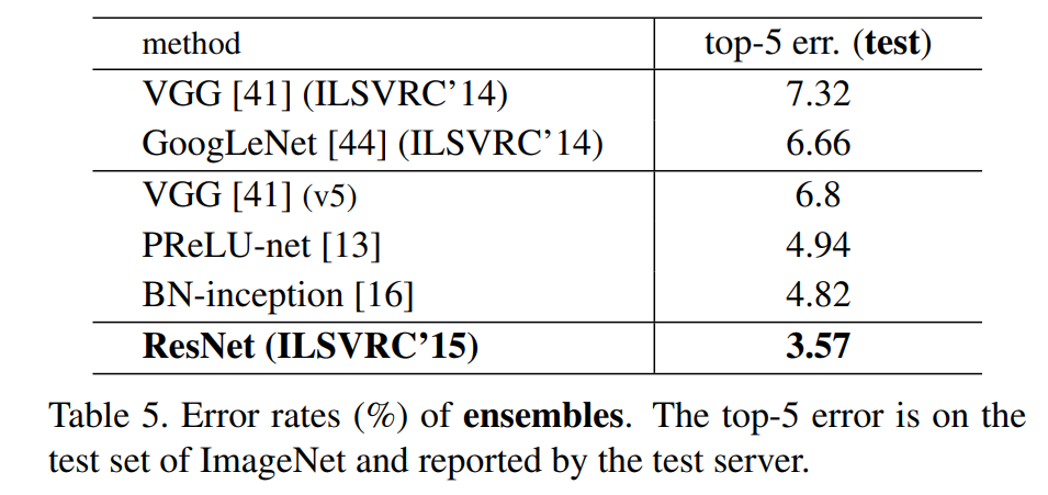
We combine six models of different depth to form an ensemble(only with two 152-layer ones at the time of submitting). This leads to 3.57% top-5 error on the test set . This entry won the 1st place in ILSVRC 2015.
결과적으로 위에서 만들었던 6가지의 모델을 앙상블을 해서 top-5 error 3.57%까지 줄였고 이 모델이 ILSVRC 2015에서 우승했다.

CIFAR-10 and Analysis

We conducted more studies on the CIFAR-10 dataset, which consists of 50k training images and 10k testing images in 10 classes. We present experiments trained on the training set and evaluated on the test set.
CIFAR-10 dataset에도 실험을 하였는데 이 dataset의 5만장의 이미지는 training, 1만장의 이미지를 test에 적용했으며 10개의 클래스를 가지고 있다.
Our focus is on the behaviors of extremely deep networks, but not on pushing the state-of-the-art results, so we intentionally use simple architectures as follows.
우리는 극도로 깊은 layer에 대해서
The plain/residual architectures follow the form in Fig. 3 (middle/right). The network inputs are 32×32 images, with the per-pixel mean subtracted.
검증 방식은 동일한 layer 수를 갖는 Plain과 Residual Network을 비교 실험하는 한다. CIFAR-10의 영상은 크기가 매우 작기 때문에, 맨 처음 convolutional layer에 3x3 kernel을 썼으며 이미지의 평균을 각 픽셀에서 빼주는 정규화 작업을 진행했다.
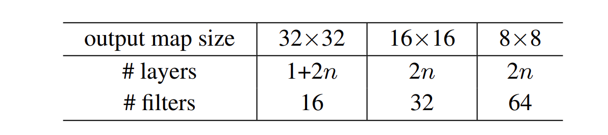
The first layer is 3×3 convolutions. Then we use a stack of 6n layers with 3×3 convolutions on the feature maps of sizes {32, 16, 8} respectively, with 2n layers for each feature map size. The numbers of filters are {16, 32, 64} respectively.
처음에는 3x3 convolutional layer 수행 후 3x3 Convolution layer를 6n개의 쌓는다. 그 6n 중 각각의 2n에 대하여 feature map의 크기가 {32, 16, 8}이 되도록 하였으며, filter의 개수는 연산량의 균형을 맞춰주기 위해 {16, 32, 64}가 되도록 하였다.
The subsampling is performed by convolutions with a stride of 2.
subsampling(=downsampling)은 stride=2의 convolution을 통해 수행된다,
The network ends with a global average pooling, a 10-way fully-connected layer, and softmax.
맨 마지막에는 global average pooling과 10의 class를 분류하는 fully connected layer를 배치하였다.
There are totally 6n+2 stacked weighted layers.
결과적으로 전체 layer수는 6n+2가 된다.
The following table summarizes the architecture:
아래 테이블은 아키텍처를 요약한 표이다.

When shortcut connections are used, they are connected to the pairs of 3×3 layers (totally 3n shortcuts)
shortcut connection을 이용하게 되면, 한 쌍의 3 x 3 Layer에 연결된다. (총 3n개의 shortcut)
On this dataset we use identity shortcuts in all cases (i.e., option A), so our residual models have exactly the same depth, width, and number of parameters as the plain counterparts.
해당 Dataset에서는 모든 경우에 identity shortcut을 사용했으며, 제안된 residual model들은 모두 같은 depth, width, parameter 개수를 갖는다.
We use a weight decay of 0.0001 and momentum of 0.9, and adopt the weight initialization in and BN but with no dropout. These models are trained with a minibatch size of 128 on two GPUs. We start with a learning rate of 0.1, divide it by 10 at 32k and 48k iterations, and terminate training at 64k iterations, which is determined on a 45k/5k train/val split. We follow the simple data augmentation in for training: 4 pixels are padded on each side, and a 32×32 crop is randomly sampled from the padded image or its horizontal flip. For testing, we only evaluate the single view of the original 32×32 image.
실험에 사용한 environment들은 다음과 같다.
Data argumentation: 4 pixel padded on each side & 32 x 32 crop is randomly sampled from the padded image or its horizontal flip
Batch Normalization: O
Batch size: 128 on two GPUs
Learning rate: 0.1 (divided by 10 at 32k and 48k iterations, and terminate training at 64k)
Wight Decay: 0.0001 (Momentum of 0.9)
Dropout: X

We compare n = {3, 5, 7, 9}, leading to 20, 32, 44, and 56-layer networks. Fig. 6 (left) shows the behaviors of the plain nets.

본 논문에서는 n이 각각 3, 5, 7, 9일 때, 20, 32, 44, 56개의 Layer로 이루어진 모델들을 비교했다.

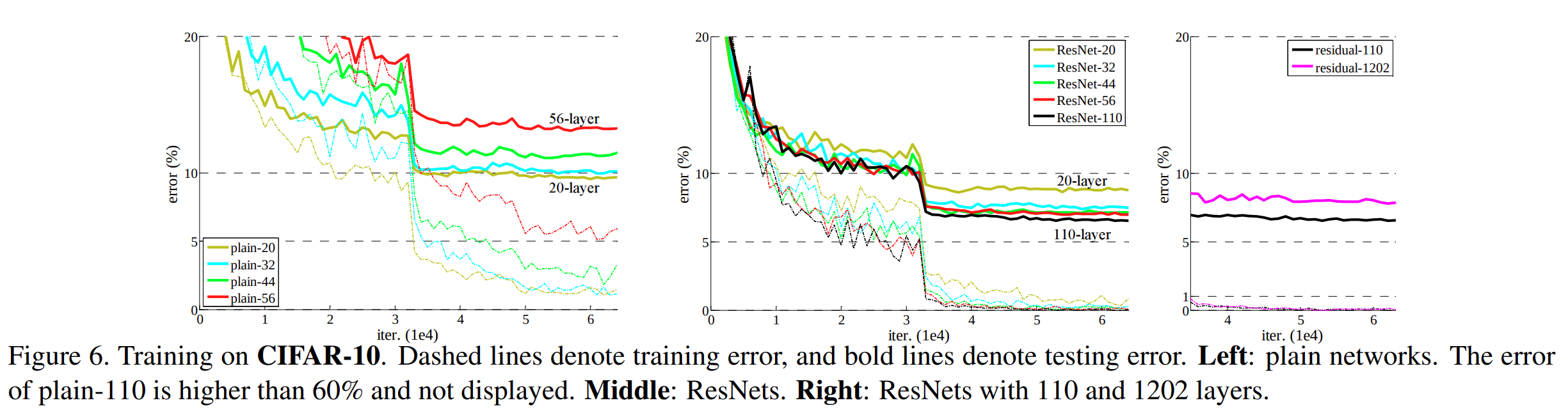
가장 왼쪽부터 차례대로 Plain network, ResNet, ResNet110, 1202 Layers이다.
먼저 왼쪽의 Plain Network 그림을 보자.
The deep plain nets suffer from increased depth, and exhibit higher training error when going deeper. This phenomenon is similar to that on ImageNet and on MNIST, suggesting that such an optimization difficulty is a fundamental problem.
모델의 깊이가 깊어질수록 training error가 증가하며, 앞서 설명한 ImageNet과 MNIST 데이터 셋과 비슷한 현상이 나타나는 것을 확인할 수 있다.
Fig. 6 (middle) shows the behaviors of ResNets. Also similar to the ImageNet cases (Fig. 4, right), our ResNets manage to overcome the optimization difficulty and demonstrate accuracy gains when the depth increases.
가운데는 ResNet의 양상을 보여주는 그림이다. 이 또한 ImageNet의 결과와 비슷하며, 최적화의 어려움과 깊이가 깊어질수록 정확도가 감소하는 문제를 해결했다.
마지막 그림은 ResNet 110, 1202 Layers의 양상을 보여주는 그림이다.
We further explore n = 18 that leads to a 110-layer ResNet. In this case, we find that the initial learning rate of 0.1 is slightly too large to start converging. So we use 0.01 to warm up the training until the training error is below 80% (about 400 iterations), and then go back to 0.1 and continue training.
이처럼 굉장히 깊은 Layer의 경우, 초기에 설정한 learning rate는 0.1이 수렴하기에는 너무 큰 값이기에, Training error가 80%(약 400 iterations) 미만이 될 때까지는 0.01을 사용했다.
The rest of the learning schedule is as done previously. This 110-layer network converges well.
나머지 학습 환경은 이전과 동일하다. 그 결과 모델이 잘 수렴하는 것으로 나타났다.
It has fewer parameters than other deep and thin networks such as FitNet and Highway(Table 6), yet is among the state-of-the-art results (6.43%, Table 6).
이 모델의 경우 다른 FitNet, Highway보다 적은 파라미터 수를 가졌고, 더 높은 성능을 보였다.

Analysis of Layer Responses.

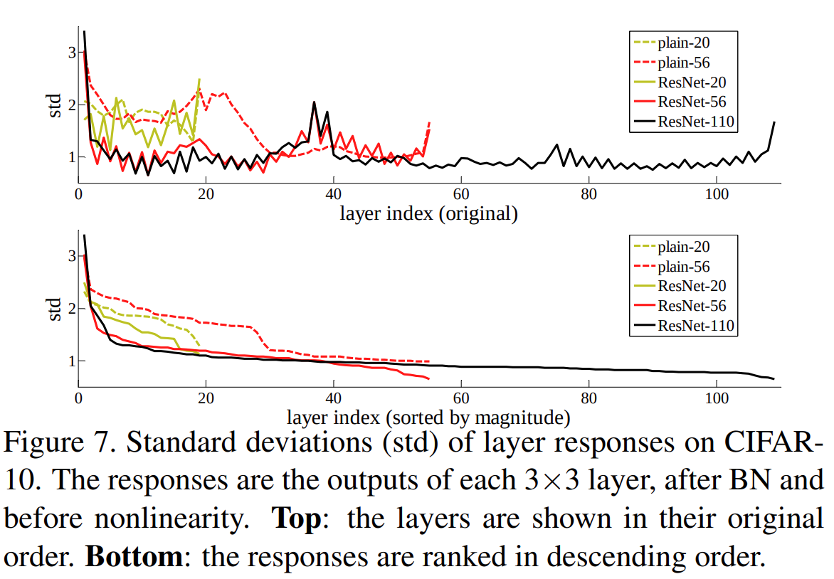
Fig. 7 shows the standard deviations (std) of the layer responses.
위 그림은 Layer responses의 standard deviations(std) 를 나타낸다.
The responses are the outputs of each 3×3 layer, after BN and before other nonlinearity (ReLU/addition).
여기서 response 는 각 3x3 Layer의 결과로, BN 이후와 nonlinearity(RELU/addition) 이전이다.
For ResNets, this analysis reveals the response strength of the residual functions.
ResNet에서, 이 분석값은 residual function의 response 강도를 나타낸다.
Fig. 7 shows that ResNets have generally smaller responses than their plain counterparts.
Fig 7. 을 보면, ResNet은 일반적으로 Plain Net보다 작은 response를 보였다.
These results support our basic motivation(Sec.3.1) that the residual functions might be generally closer to zero than the non-residual functions.
이는 앞서 얘기했던 non-residual function보다 residual function이 0에 더 가깝다는 점과 동일하다.
We also notice that the deeper ResNet has smaller magnitudes of responses, as evidenced by the comparisons among ResNet-20, 56, and 110 in Fig. 7.
ResNet 20, 56, 110을 비교해보면, 더 깊은 ResNet이 더 작은 response를 가진다는 것 또한 알 수 있다.
When there are more layers, an individual layer of ResNets tends to modify the signal less.
즉, Layer가 깊어질수록 signal이 적게 변화하는 경향이 나타났다.

Exploring Over 1000 layers

We explore an aggressively deep model of over 1000 layers. We set n = 200 that leads to a 1202-layer network, which is trained as described above.
그렇다면 1000개 이상의 Layer를 가진 아주 깊은 모델은 어떨지 탐구한다. 앞선 Figure 6. 에서 언급된 n = 200 인 1202-Layer network를 보자.
The testing result of this 1202-layer network is worse than that of our 110-layer network, although both have similar training error.
비교적 더 얕은 모델인 110-Layer의 경우와 1202-layer network의 Training Error는 비슷하지만, Testing Error는 더 깊은 모델인 1202-Layer가 더 안좋은 것을 확인할 수 있다.
But there are still open problems on such aggressively deep models.
그러나 1202-Layer처럼 매우 깊은 모델에 대해서는 여전히 학습이 잘 되지 않는 문제가 있다.
We argue that this is because of overfitting.
해당 현상의 원인은 overfitting을 주장한다.
The 1202-layer network may be unnecessarily large (19.4M) for this small dataset.
그 이유는 1202-Layer는 작은 dataset에 비해 필요이상으로 크기 때문이다.
Strong regularization such as maxout or dropout is applied to obtain the best results ([10, 25, 24, 35]) on this dataset.
maxout, dropout과 같은 강한 Regularization이 좋은 결과를 내보였다.
In this paper, we use no maxout/dropout and just simply impose regularization via deep and thin architectures by design, without distracting from the focus on the difficulties of optimization.
그러나 해당 논문에서는 이러한 기법들을 사용하지 않고 깊으면서도 thin architectures를 통한 간단한 정규화 방법을 사용하였다.
But combining with stronger regularization may improve results, which we will study in the future.
다만, 더 강력한 정규화 기법을 결합하면 결과를 개선할 수 있을 것으로 보이며, 이에 대해서는 미래의 연구에서 살펴볼 예정이다.

Object Detection on PASCAL and MS COCO

Our method has good generalization performance on other recognition tasks.
해당 method는 recognition에서도 좋은 성능을 보였다.
Table 7 and 8 show the object detection baseline results on PASCAL VOC 2007 and 2012 and COCO.
위 Table 7, Table 8.은 PASCAL VOC 2007, 2012, COCO Dataset와 같은 객체 검출 결과이다.
We adopt Faster R-CNN as the detection method. Here we are interested in the improvements of replacing VGG-16 [41] with ResNet-101.
Detection method로는 Faster R-CNN 모델을 사용했으며, VGG-16을 ResNet-101로 교체했다. Most remarkably, on the challenging COCO dataset we obtain a 6.0% increase in COCO’s standard metric mAP@[.5, .95]) which is a 28% relative improvement.
놀랍게도 COCO dataset challenging에서 6.0%증가 하여 28%의 상대적인 개선을 보여준다.
ResNet이 Representation을 잘 학습하여 성능이 향상된 것을 확인할 수 있다.
Based on deep residual nets, we won the 1st places in several tracks in ILSVRC & COCO 2015 competitions: ImageNet detection, ImageNet localization, COCO detection, and COCO segmentation. The details are in the appendix
이러한 깊은 Residual Net을 기반으로, ILSVRC & COCO 2015 대화에서 1위를 차지했다. 해당 대회에서는 ImageNet detection, ImageNet localization, COCO detection, 그리고 COCO segmentation이 있다. 더 자세한 내용은 논문의 부록에서 확인할 수 있다.

ResNet 논문리뷰

서론

목차

Abstact

Introduction

Research background

Recent Research

Convergence Problem

Degradation Problem

Summary

Propose

Summary

Related Work

Residual Representation

VLAD & Fisher Vector

Short Connections

Deep Residual Learning

3.1 Residual learning

3.2 Identity Mapping by Shortcuts

3.3 Network Architectures

3.4 Implementation

Experiments

ImageNet Classification

Plain Networks

Residual Networks

Identity vs. Projection Shortcuts

Deeper Bottleneck Architectures

50-layer ResNet

101-layer and 152-layer ResNets

Comparisons with State-of-the-art Methods

CIFAR-10 and Analysis

Analysis of Layer Responses.

Exploring Over 1000 layers

Object Detection on PASCAL and MS COCO

Comment