
서론
이 장은 Image의 채널이 어떤식으로 픽셀에서 자리잡고(위치) 있는지 확인해보고 직접 픽셀별 출력해보는 실습을 진행한다.
목차
- 가상의 Array를 생성하고 shape 확인해보기
- ⚠️Library별 shape 표기
- Real Image shape 확인해보기
- Pytorch의 Shape
- Channel별 이미지 출력해보기
- CV2로 이미지 채널별 출력하기
가상의 Array를 생성하고 shape 확인해보기
2D Array
다음과 같은 2차원의 배열을 만들고 shape을 찍어보자.
test = np.array([
    [1, 2, 3],
    [4, 5, 6],
    [7, 8, 9],
    [10, 11, 12]
])

# print(test)
# print(test.shape) # (4, 3)
결과: (4, 3)
3D Array
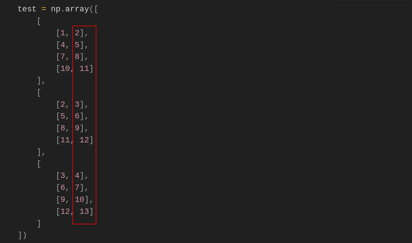
3차원의 배열을 만들고 찍어보자
test = np.array([
    [
        [1, 2],
        [4, 5],
        [7, 8],
        [10, 11]
    ],
    [
        [2, 3],
        [5, 6],
        [8, 9],
        [11, 12]
    ],
    [
        [3, 4],
        [6, 7],
        [9, 10],
        [12, 13]
    ]
])

print(test)
print(f"test.shape{test.shape}") # (2, 4, 3)
결과: (3, 4, 2)
그럼 (2, 4)의 크기를 갖는 2채널을 갖는 이미지라 가정하고 0번째 채널을 찍어보자.
print(f"0-channel: \n{test[:,:,0]}")결과 :
test.shape(3, 4, 2)
0-channel:
[[ 1  4  7 10]
 [ 2  5  8 11]
 [ 3  6  9 12]]
즉 아래 열을 쭉 나열한 것을 볼 수 있다.
두번째 채널을 찍어보자.
print(f"1-channel: \n{test[:,:,1]}")결과:
test.shape(3, 4, 2)
1-channel:
[[ 2  5  8 11]
 [ 3  6  9 12]
 [ 4  7 10 13]]
이번에는 두번째 열을 쭉 나열한 것을 볼 수 있다.
그럼 여기서 이미지가 3채널이라면 하나의 열이 추가적으로 생성될 것이라는 것을 알 수 있다.
실제 이미지를 불러와서 확인해보자.
⚠️Library별 shape 표기
Real Image shape 확인해보기
먼저 이미지를 읽고 numpy array로 변경해보겠다.
image = Image.open('./1.jpg')
image = image.resize((5, 6))
image = np.array(image)
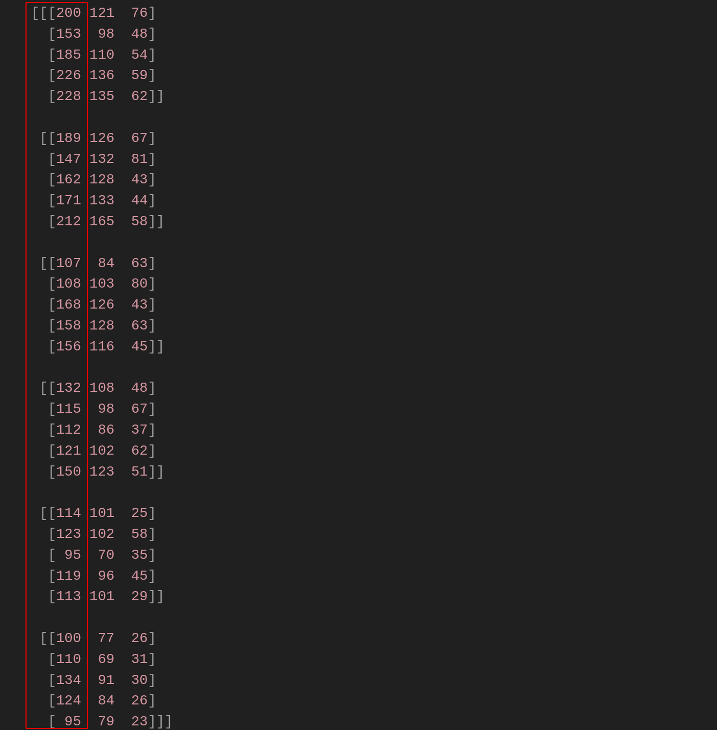
print(f"numpy-image: {image.shape}") # numpy-image: (6, 5, 3)Print out 3-channel Image Pixel
[[[200 121  76]
  [153  98  48]
  [185 110  54]
  [226 136  59]
  [228 135  62]]

 [[189 126  67]
  [147 132  81]
  [162 128  43]
  [171 133  44]
  [212 165  58]]

 [[107  84  63]
  [108 103  80]
  [168 126  43]
  [158 128  63]
  [156 116  45]]

 [[132 108  48]
  [115  98  67]
  [112  86  37]
  [121 102  62]
  [150 123  51]]

 [[114 101  25]
  [123 102  58]
  [ 95  70  35]
  [119  96  45]
  [113 101  29]]

 [[100  77  26]
  [110  69  31]
  [134  91  30]
  [124  84  26]
  [ 95  79  23]]]
Check red-channel pixel place
0번째 채널인 R채널을 출력해보면 다음과 같은 위치에 출력된다.
image = Image.open('./1.jpg')
image = image.resize((5, 6)) # 세로(height), 가로(width)
image = np.array(image)
print(image)
red_channel = image[:, :, 0]
print('='*100)
print(red_channel)
결과:
[[200 153 185 226 228]
 [189 147 162 171 212]
 [107 108 168 158 156]
 [132 115 112 121 150]
 [114 123  95 119 113]
 [100 110 134 124  95]]
Array를 가상으로 만든 것과 마찬가지로 R채널에 해당되는 픽셀값들은 아래와 같은 곳에서 모아짐을 알 수 있다.
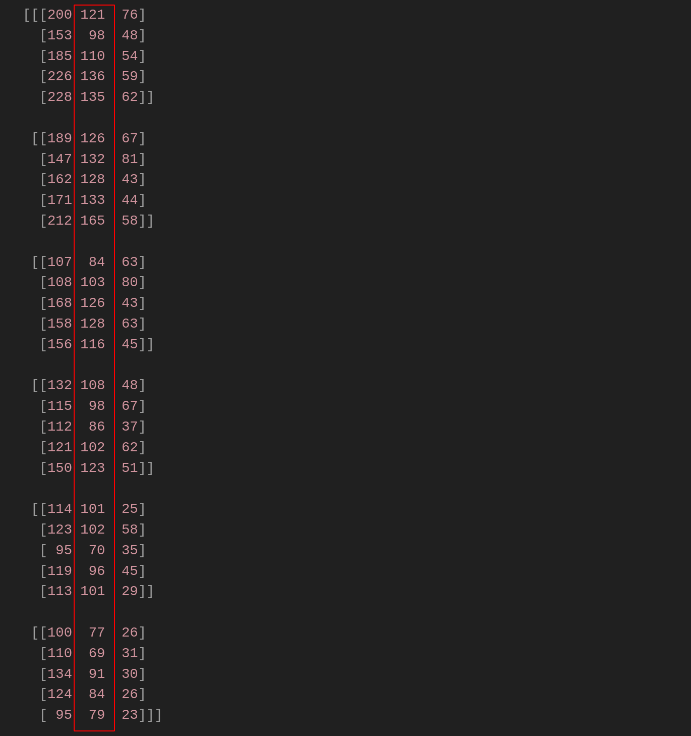
Check green-channel pixel place
1번째 채널인 B채널을 출력해보면 다음과 같은 위치에 출력된다.
image = Image.open('./1.jpg')
image = image.resize((5, 6)) # 세로(height), 가로(width)
image = np.array(image)
print(image)
green_channel = image[:, :, 1]
print('='*100)
print(green_channel)
결과:
[[121  98 110 136 135]
 [126 132 128 133 165]
 [ 84 103 126 128 116]
 [108  98  86 102 123]
 [101 102  70  96 101]
 [ 77  69  91  84  79]]
Array를 가상으로 만든 것과 마찬가지로 G채널에 해당되는 픽셀값들은 아래와 같은 곳에서 모아짐을 알 수 있다.
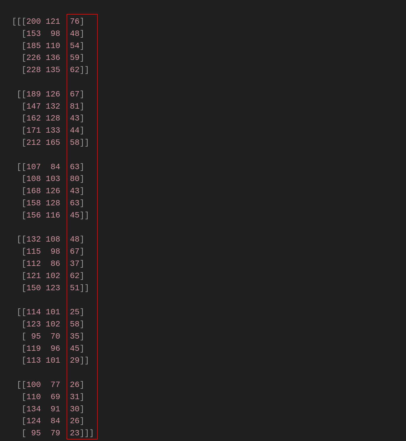
Check blue-channel pixel place
2번째 채널인 B채널을 출력해보면 다음과 같은 위치에 출력된다.
image = Image.open('./1.jpg')
image = image.resize((5, 6)) # 세로(height), 가로(width)
image = np.array(image)
print(image)
blue_channel = image[:, :, 2]
print('='*100)
print(blue_channel)
결과:
[[76 48 54 59 62]
 [67 81 43 44 58]
 [63 80 43 63 45]
 [48 67 37 62 51]
 [25 58 35 45 29]
 [26 31 30 26 23]]
Array를 가상으로 만든 것과 마찬가지로 G채널에 해당되는 픽셀값들은 아래와 같은 곳에서 모아짐을 알 수 있다.
Pytorch의 Shape
numpy 배열에서는 일반적으로 이미지 데이터는 (h, w, c) 형식으로 표현되지만, PyTorch에서는 (c, h, w) 형식으로 표현된다.
앞서 설명한 각 열의 값들을 모아서 channel을 형성한 것을 생각하면서 transpose로 shape을 변경해보자.
import numpy as np
import torch
torch.manual_seed(42)
arr = np.random.randint(0, 10, size=(2, 4, 3)) # (h, w, c)
print(arr.shape)
print(arr)
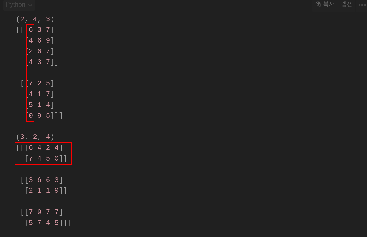
transpose_arr = np.transpose(arr,(2, 0, 1)) # (c, h, w)
print(transpose_arr.shape)
print(transpose_arr)결과:
(2, 4, 3)
[[[6 3 7]
  [4 6 9]
  [2 6 7]
  [4 3 7]]

 [[7 2 5]
  [4 1 7]
  [5 1 4]
  [0 9 5]]]

(3, 2, 4)
[[[6 4 2 4]
  [7 4 5 0]]

 [[3 6 6 3]
  [2 1 1 9]]

 [[7 9 7 7]
  [5 7 4 5]]]
다음과 같이 변경된 것을 볼 수 있다
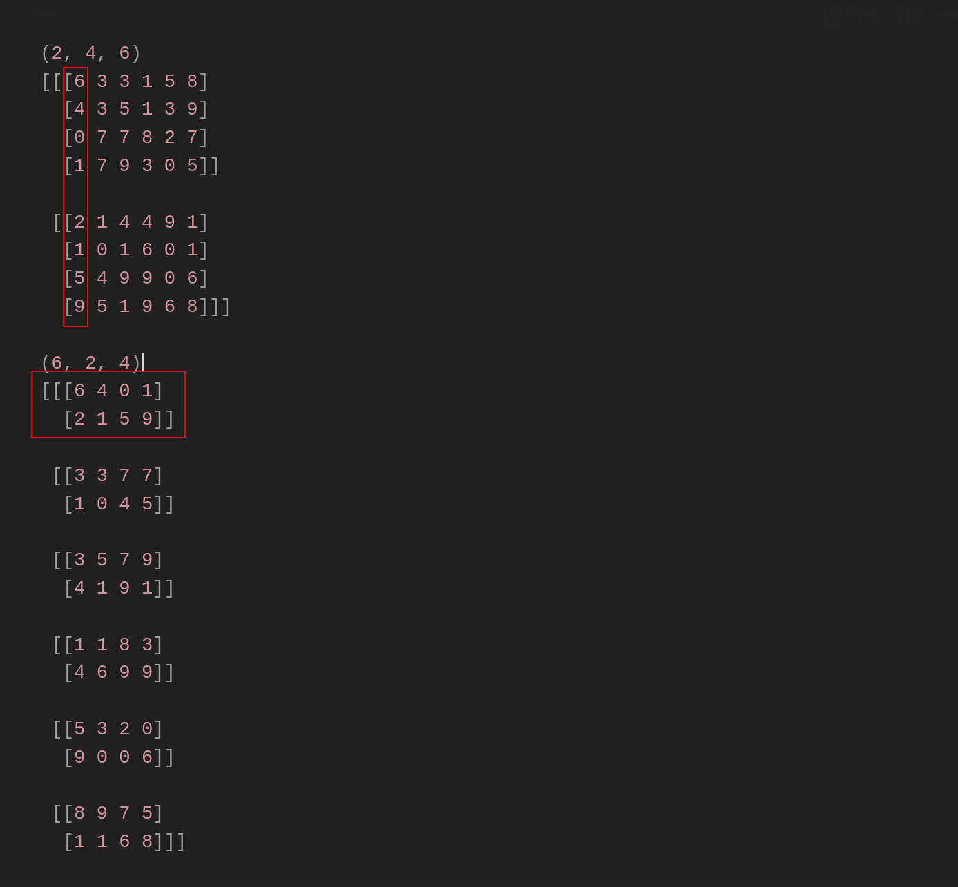
그럼 이번엔 (2, 4, 3)이 아닌 (2, 4, 6)의 Dimension을 봐보자. (수정)
arr = np.random.randint(0, 10, size=(2, 4, 6)) # (h, w, c)
print(arr.shape)
print(arr)
transpose_arr = np.transpose(arr,(2, 0, 1))
print(transpose_arr.shape)
print(transpose_arr)
결과:
채널이 6개로 늘어나면서 6개의 열이 생긴 것을 볼 수 있다.
(2, 4, 6)
[[[6 3 3 1 5 8]
  [4 3 5 1 3 9]
  [0 7 7 8 2 7]
  [1 7 9 3 0 5]]

 [[2 1 4 4 9 1]
  [1 0 1 6 0 1]
  [5 4 9 9 0 6]
  [9 5 1 9 6 8]]]

(6, 2, 4)
[[[6 4 0 1]
  [2 1 5 9]]

 [[3 3 7 7]
  [1 0 4 5]]

 [[3 5 7 9]
  [4 1 9 1]]

 [[1 1 8 3]
  [4 6 9 9]]

 [[5 3 2 0]
  [9 0 0 6]]

 [[8 9 7 5]
  [1 1 6 8]]]
각 열들이 하나의 Matrix로 이뤄져 채널을 형성하는 모습을을 볼 수 있다.
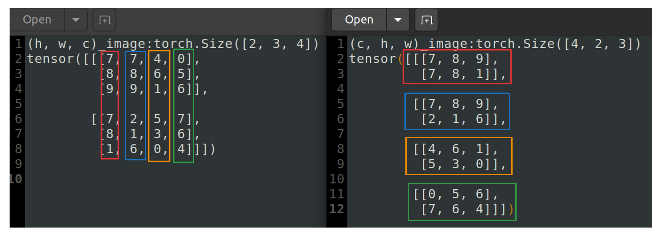
Transpose
(h, w, c)를 가지는 (2, 3, 4) 형태의 Matrix를 Transpose 시켜서 (4, 3, 2) 형태로 만들어보자
arr = np.random.randint(0, 10, size=(2, 3, 4)) # (h, w, c)
arr = torch.tensor(torch.tensor(arr))
print(f"(h, w, c)_image:{arr.shape}")
print(arr)

print('='*50)
transpose_arr = np.transpose(arr,(2, 0, 1)) # (4, 3, 2)
print(f"(c, h, w)_image:{transpose_arr.shape}")
print(transpose_arr)
결과:
(h, w, c)_image:torch.Size([2, 3, 4])
tensor([[[7, 7, 4, 0],
         [8, 8, 6, 5],
         [9, 9, 1, 6]],

        [[7, 2, 5, 7],
         [8, 1, 3, 6],
         [1, 6, 0, 4]]])
==================================================
(c, h, w)_image:torch.Size([4, 2, 3])
tensor([[[7, 8, 9],
         [7, 8, 1]],

        [[7, 8, 9],
         [2, 1, 6]],

        [[4, 6, 1],
         [5, 3, 0]],

        [[0, 5, 6],
         [7, 6, 4]]])
아래 처럼 각 열이(채널)이 Matrix형태로 변환되는 것을 볼 수 있다.
Channel별 이미지 출력해보기
matplotlib(plt)의imshow함수는 입력 받은 데이터를 color map으로 설정한 색상으로 변환된다.- 기본 컬러 맵은
viridis(녹색 계열)을 사용하며 따로 cmap을 지정해주 않으면 모든 채널 이미지가 같은 색상(녹색 계열)으로 보이게 된다. - 각 채널을 해당 색상으로 표시하기 위해서는
cmap인자를 사용해 적절한 컬러 맵을 지정해야 한다.
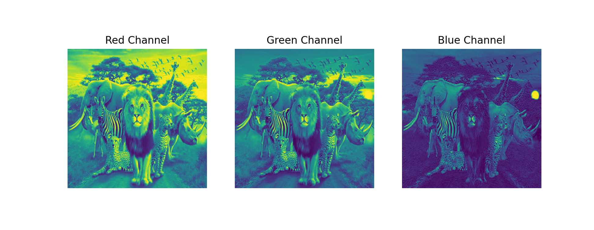
따라서 다음과 같이 cmap을 지정해주지 않을 경우 아래 처럼 이미지가 표시된다.
cmap을 지정하지 않은 경우
import matplotlib.pyplot as plt
from PIL import Image
import numpy as np

image = Image.open('./1.jpg')
image = image.resize((300, 300))
image = np.array(image)

red_channel = image[:, :, 0]
green_channel = image[:, :, 1]
blue_channel = image[:, :, 2]

fig, axs = plt.subplots(1, 3, figsize=(10, 4))

axs[0].imshow(red_channel)
axs[0].set_title('Red Channel')
axs[0].axis('off')

axs[1].imshow(green_channel)
axs[1].set_title('Green Channel')
axs[1].axis('off')

axs[2].imshow(blue_channel)
axs[2].set_title('Blue Channel')
axs[2].axis('off')

plt.show()
결과:
cmap을 지정한 경우
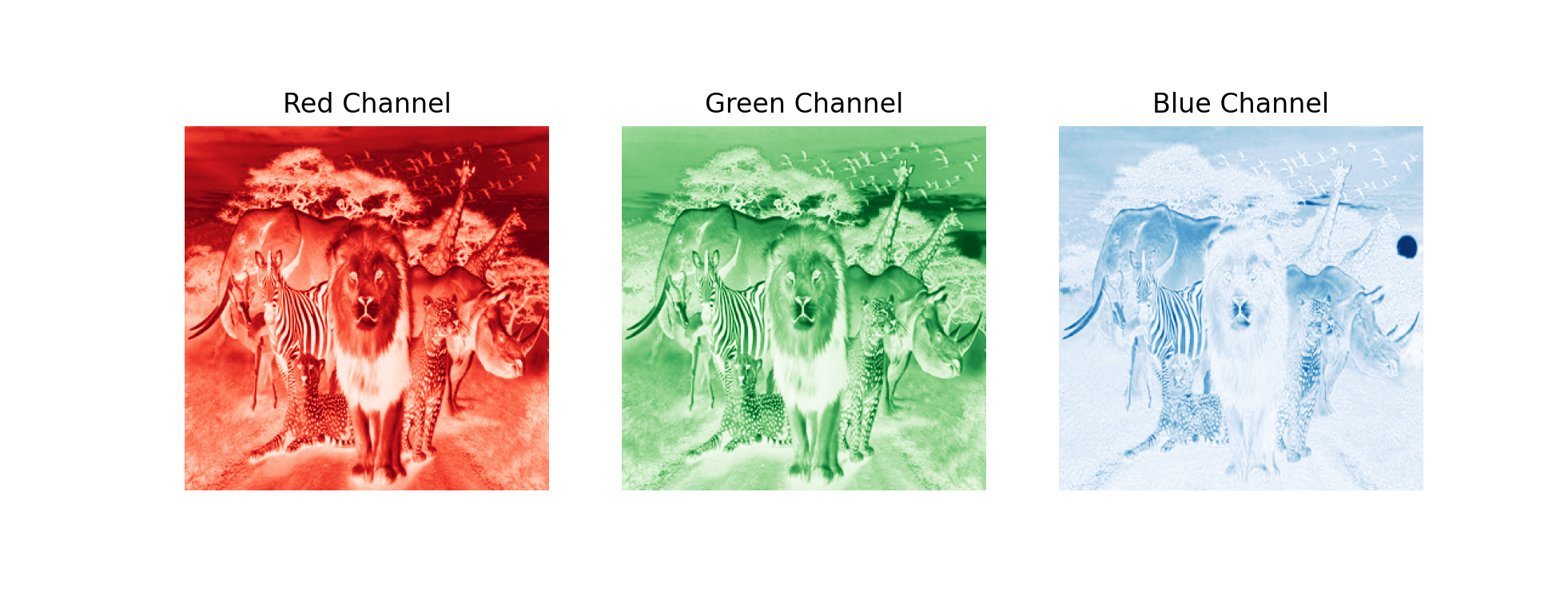
예를 들어, cmap='Reds' 을 사용하면 0의 값은 흰색에 가깝고, 1의 값은 빨간색에 가깝다. 따라서 분리된 각 채널의 픽셀값이 클수록 색상이 더 짙은 빨간색으로 표시된다.
import matplotlib.pyplot as plt
from PIL import Image
import numpy as np

image = Image.open('./1.jpg')
image = image.resize((300, 300))
image = np.array(image)

red_channel = image[:, :, 0]
green_channel = image[:, :, 1]
blue_channel = image[:, :, 2]

fig, axs = plt.subplots(1, 3, figsize=(10, 4))

axs[0].imshow(red_channel, cmap='Reds')
axs[0].set_title('Red Channel')
axs[0].axis('off')

axs[1].imshow(green_channel, cmap='Greens')
axs[1].set_title('Green Channel')
axs[1].axis('off')

axs[2].imshow(blue_channel, cmap='Blues')
axs[2].set_title('Blue Channel')
axs[2].axis('off')
결과:
CV2로 이미지 채널별 출력하기
matplotlib의 imshow의 특성 때문에 cmap의 색상을 일일이 지정해줘야 했다.
그럼 OpenCV의 경우는 어떨까?
import cv2
import numpy as np
# 이미지를 불러온다.
img = cv2.imread('1.jpg')
# 이미지를 BGR 형태로 분리한다.
b, g, r = cv2.split(img)
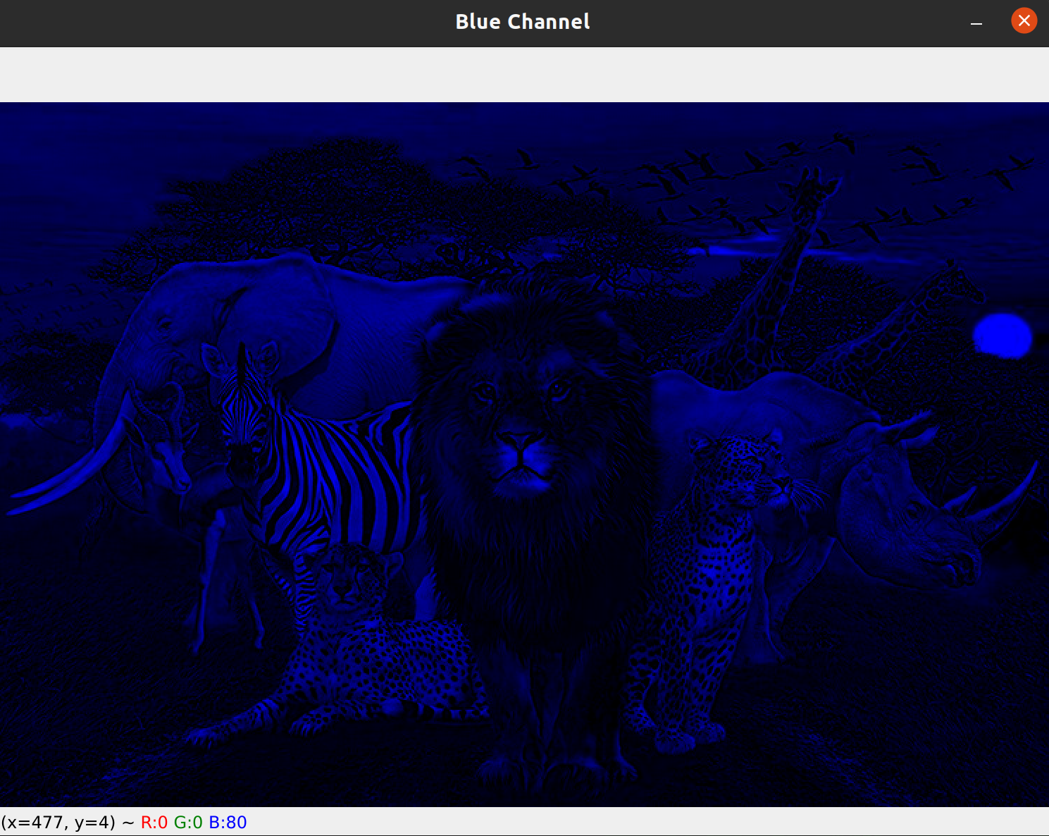
# Blue 채널을 보여주는 이미지를 만든다.
blue_img = cv2.merge([b, np.zeros_like(b), np.zeros_like(b)])
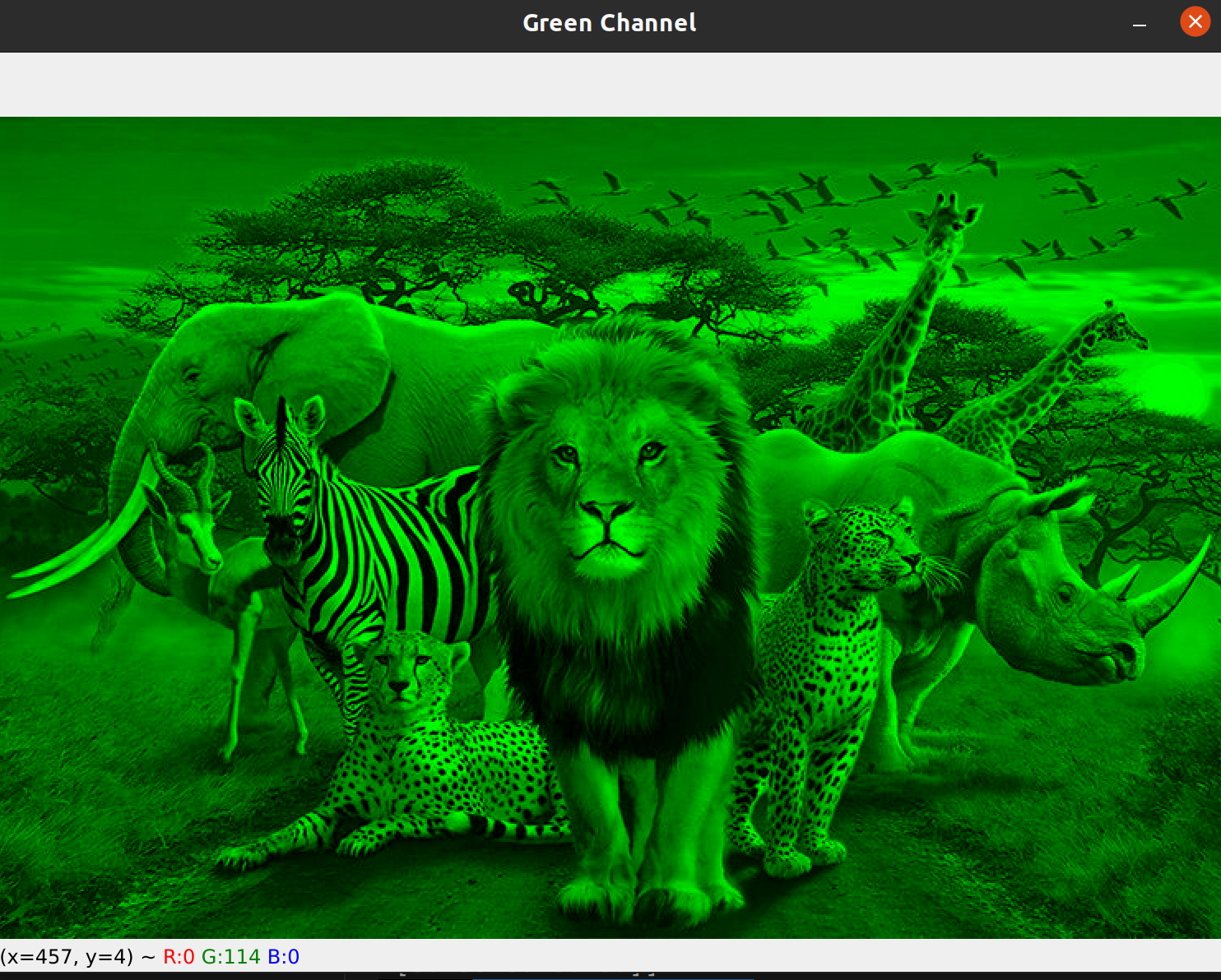
# Green 채널을 보여주는 이미지를 만든다.
green_img = cv2.merge([np.zeros_like(g), g, np.zeros_like(g)])
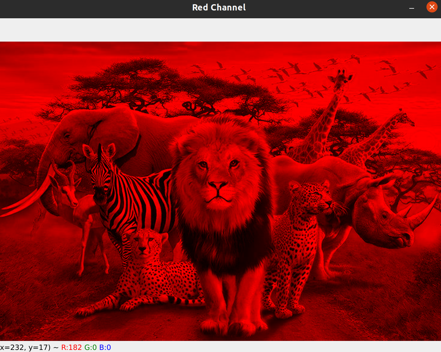
# Red 채널을 보여주는 이미지를 만든다.
red_img = cv2.merge([np.zeros_like(r), np.zeros_like(r), r])
# 이미지를 보여준다.
cv2.imshow('Blue Channel', blue_img)
cv2.imshow('Green Channel', green_img)
cv2.imshow('Red Channel', red_img)
cv2.waitKey(0)
cv2.destroyAllWindows()zeros는 말 그대로 zero들로 가득찬 array를 만든다.
test = np.zeros([3, 5])
print(test)
# 결과:
[[0. 0. 0. 0. 0.]
 [0. 0. 0. 0. 0.]
[0. 0. 0. 0. 0.]]zeros_like는 어떤 특정 array와 같은(like) 사이즈(size), 크기(shape)의 zeros array를 만든다.
test = np.zeros([3, 5])
print(np.zeros_like(test))
# 결과:
[[0. 0. 0. 0. 0.]
 [0. 0. 0. 0. 0.]
 [0. 0. 0. 0. 0.]]
blue_img = cv2.merge([b, np.zeros_like(b), np.zeros_like(b)]) 는 b, g, r 로 구성된 openCV의 경우에 b-channel을 제외한 g, r채널을 0으로 만들어 주는 것이다.
따라서 3채널의 이미지이지만 g, r채널을 다 0으로 만들어줌으로써 b채널의 값만 보이게 된다.
Comment