MonoLift: Learning 3D Manipulation Policies from Monocular RGB via Distillation

서론

이 논문은 단일 RGB 이미지(Monocular RGB)만으로 3D 로봇 조작 정책을 학습하는 MonoLift framework를 제안한다.

기존 RGB-D, multi-view, point cloud 기반 방법은 3D 정보를 잘 활용할 수 있지만, 추가 센서와 전처리 비용이 크다. 반대로 RGB-only 방식은 배포가 쉽지만 깊이 정보가 없어 3D 위치 차이를 구분하기 어렵고, 이로 인해 부정확한 action을 출력할 수 있다.

MonoLift는 이를 해결하기 위해 학습 단계에서만 Depth Anything V2로 만든 pseudo-depth를 사용하는 teacher model을 만들고, 이 teacher의 3D-aware knowledge를 RGB-only student model에게 전달한다.

전달되는 지식은 크게 세 가지이다.

Spatial knowledge: RGB만으로도 3D 공간 구조를 이해하도록 함
Temporal knowledge: 시간에 따른 상태 변화를 안정적으로 이해하도록 함
Action knowledge: teacher의 3D-aware action 선택을 따라가도록 함

즉, MonoLift는 학습 중에는 depth 정보를 활용하지만, 실제 배포 시에는 depth estimator 없이 RGB-only로 동작하는 효율적인 3D manipulation policy 학습 방법이다.

Problem Formulation

이 논문에서 목표는 단일 RGB 이미지와 언어 명령을 입력으로 받아 로봇 조작 action을 출력하는 policy를 학습하는 것이다.

하나의 학습 데이터 \(\tau_i\)는 무엇을 해야 하는지 알려주는 언어 명령 \(g_i\)와 그 명령을 수행하는 동안 시간별로 저장된 이미지 \(o_t^i\)와 expert action \(a_t^i\)의 쌍 으로 구성되며 다음과 같이 표현된다.

\tau_i = \left(g_i,{(o_t^i,a_t^i)}_{t=1}^{T}\right)

\(g_i\): language instruction(입력 이미지 명령)
- example) 컵을 잡아라
\(o_t^i\): t시점에서의 관측 RGB 이미지
\(a_t^i\): t시점에서의 Target(expert) action
\(T\): instruction을 수행하는 한 에피소드 길이
\(\mathcal{D} = \{\tau_i\}_{i=1}^N\): 전체 demonstration dataset
- 여러 행동 명령에 따른 트라젝토리

이 논문의 학습 목표는 관측 이미지와 instruction이 주어졌을때 Target action을 예측하도록 신경망을 학습시키는 것이다.

\pi_{\theta}(a_t|o_t,\;g)

Spatial Representation Distillation

Teacher와 Student를 함께 end-to-end로 학습한다.

Teacher는 RGB image에 pseudo-depth map을 추가하여 더 강한 3D-aware representation을 만드는 것이다.

teacher가 Depth Anything V2를 사용하여 RGB image로부터 pseudo-depth map을 생성한다.

Student는 Inference에서 RGB입력만을 사용해야 함으로 따로 깊이 맵을 사용하지 않는다.

전체 플로우는 아래 그림과 같다.

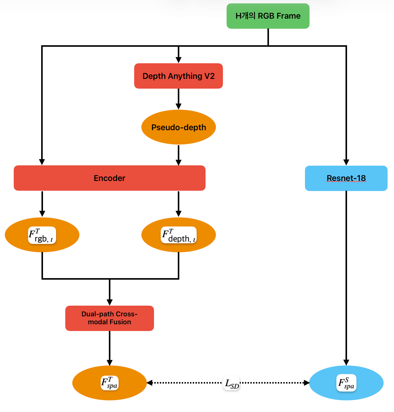
Input

\(o_{t-H+1:t}\): 최근 H개의 RGB Frame을 사용한다.

이 입력은 teacher branch와 student branch로 동시에 들어간다.

Teacher branch

Teacher는 RGB만 보지 않고 RGB에서 추정한 pseudo-depth(\(d_t\))도 함께 사용한다.

먼저 RGB Frame이 Depth Anything V2로 들어간다.

d_t = \text{DepthAnythingV2}(o_t)

그리고 H개의 RGB Frame과 \(d_t\)를

각각 동일한 encoder에 입력으로 넣는데 넣기 전에 RGB 이미지와 비슷하게 보이도록 pseudo-colored heatmap으로 변환한다.

이렇게 하는 이유는 RGB와 depth 사이의 색, 밝기, edge, texture 같은 이미지의 기초적인 겉모습(low-level appearance) 차이가 줄어들기 때문이다.

RGB image를 encoder에 넣어서 \(F^T_{\text{rgb}, t}\)를 만들고 pseudo-depth를 encoder에 넣어서 \(F^T_{\text{dep}, t}\) 를 만든다.

\(F^T_{\text{rgb}, t}\): RGB 이미지에서 얻은 색상, 물체 모양, texture, 장애물 배치 정보 등
\(F^T_{\text{dep}, t}\): pseudo-depth에서 얻은 거리. 깊이 경계, 공간 구조 정보 등

같은 encoder를 사용하는 이유는 RGB와 pseudo-depth를 같은 representation feature 기준으로 맞춰 modality gap을 줄이고, RGB-depth fusion과 student distillation을 더 안정적으로 만들기 위해서이다.

이후 두 feature를 Dual-path Cross-modal Fusion에 넣는다.

F^T_{\text{spa},\;t} = \text{Fusion}(F^T_{\text{rgb}, t},\;F^T_{\text{dep}, t})

이 레이어에서 두 feature를 결합하여 teacher의 최종 spatial feature를 만든다.

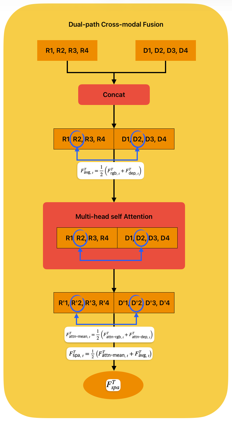
Teacher는 같은 시점 t에서 두 종류의 feature를 가진다.

F^{T}_{\text{rgb},\;t} \;,\; F^{T}_{\text{dep},\;t}

그림에서는 H개의 frame임으로 각 데이터 값을 간단하게 다음과 같이 표현한다.

\(F^{T}_{\text{rgb},\;1} = \text{R}1\)
\(F^{T}_{\text{dep},\;1} = \text{D}1\)

F^{T}_{\text{rgb},\;t} = [\text{R}1, \text{R}2,\text{R}3,\text{R}4] \\F^{T}_{\text{dep},\;t} = [\text{D}1, \text{D}2,\text{D}1,\text{D}4]

이 둘을 Concat하여 Feature를 하나로 이어붙인다.

[F^{T}_{\text{rgb},\;t},\;F^{T}_{\text{dep},\;t}]

RGB feature   = [R1, R2, R3, R4]
Depth feature = [D1, D2, D3, D4]

Concat = [R1, R2, R3, R4, D1, D2, D3, D4]

Concat된 feature는 Multi-head self-attention으로 들어간다.

F^T_{\text{attn},\;t} = \text{MHSA}\left([F^T_{\text{rgb},\;t}, F^T_{\text{dep},\;t}]\right)

Self-attention을 거치면 RGB token은 depth token을 참고하고, depth token은 RGB token을 참고한다.

즉, 장면 전체에서 RGB와 depth가 어떤 관계를 가지는지 학습하는 것이다.

Self-attention을 통과한 결과는 다시 RGB 쪽과 depth 쪽으로 나눌 수 있다.

Attention output
= [R1', R2', R3', R4', D1', D2', D3', D4']

이를 두 부분으로 나누면,

\begin{aligned}F^T_{\text{attn-rgb},\;t} &= [R1', R2', R3', R4'] \\F^T_{\text{attn-dep},\;t} &= [D1', D2', D3', D4']\end{aligned}

Self-attention을 거친 R'과 D'는 서로의 정보를 어느 정도 참고한 feature이다.

그다음 attention을 거친 RGB-side feature와 depth-side feature를 같은 위치끼리 평균낸다.

F^T_{\text{attn-mean},\;t} = \frac{1}{2}\left(F^T_{\text{attn-rgb},\;t} + F^T_{\text{attn-dep},\;t}\right)

이 결과가 attention branch에서 얻은 fusion feature이다.

동시에, 원래 RGB feature와 depth feature를 같은 위치끼리 직접 평균낸다.

이 부분은 Multi-head Self-Attention으로 들어가는 중간 결과가 아니라, attention branch와 병렬로 계산되는 feature이다. 이 부분은 같은 위치의 RGB-depth 정보를 직접 보존하는 것이다.

F^T_{\text{avg},\;t} = \frac{1}{2}\left(F^T_{\text{rgb},\;t} + F^T_{\text{dep},\;t}\right)

마지막으로 두 fusion 결과를 다시 평균낸다. 최종 feature는 전체 관계 정보 + 같은 위치의 local 구조 정보 두 가지 정보를 모두 포함한다.

Student branch

Depth를 사용하지않고 RGB Frame을 ResNet-18 Encoder에 넣는다.

F^{S}_{\text{spa},\; t} = E(o_t)

RGB만 보기 때문에 깊이 정보가 부족하다. 따라서 teacher의 \(F^{T}_{\text{spa},\; t}\)를 따라가도록 학습시킨다.

Output

Spatial Distillation Loss로 teature feature, student feature가 비슷해지도록 만든다.

L_{SD} = \frac{1}{H}\sum_{t=t_0-H+1}^{t_0}||F^{S}_{\text{spa},\; t} - F^T_{\text{spa},\;t}||^2_2

Student는 depth가 있는 것처럼 3D 구조를 반영하는 feature를 만들도록 훈련된다.

여기서 H는 frame 갯수 이다.

Temporal Dynamics Distillation

이 부분에서는 Student가 RGB만 보고도 Teacher처럼 시간에 따른 상태 변화를 이해하도록 만드는 것이다.

RGB 한 장만 보면 예를들어 “컵이 있다” 정도는 알 수 있지만, 시간 흐름을 보면 “gripper가 컵에 가까워지고 있다”, “손잡이와 정렬되고 있다”, “이제 잡아야 한다” 같은 상태 전이를 알 수 있다.

monocular RGB만으로는 이런 temporal variation이 충분하지 않기 때문에, teacher의 3D-aware temporal feature 변화량을 student가 따라가도록 학습한다.

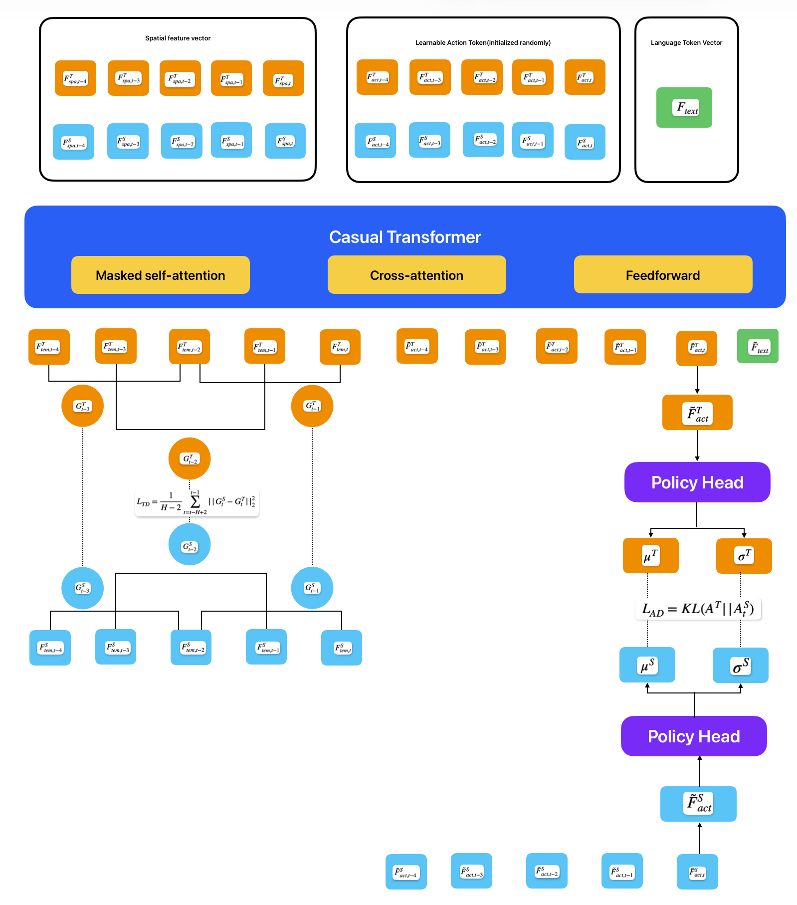
Input

입력은 순서대로 연결된 Spatial Token, Learnable action token, Language token 세 가지 종류가 입력으로 들어간다.

Spatial Token

spatial token은 장면이 어떻게 생겼는지 물체가 어디 있는지 등을 나타내는 visual feature이다.

H=5라면 입력 spatial token은 다음과 같다.

[F_{\text{spa},\;t-4}, F_{\text{spa},\;t-3}, F_{\text{spa},\;t-2}, F_{\text{spa},\;t-1}, F_{\text{spa},\;t}]

Teacher인 경우 RGB와 pseudo-depth를 fusion해서 만든 feature를 사용하고

F^T_{\text{spa},\;t}

Student는 RGB만 보고 만든 feature를 사용한다.

F^S_{\text{spa},\;t}

teacher쪽 입력은 다음과 같다.

[F^T_{\text{spa},\;t-4}, F^T_{\text{spa},\;t-3}, F^T_{\text{spa},\;t-2}, F^T_{\text{spa},\;t-1}, F^T_{\text{spa},\;t}]

student쪽 입력은 다음과 같다.

[F^S_{\text{spa},\;t-4}, F^S_{\text{spa},\;t-3}, F^S_{\text{spa},\;t-2}, F^S_{\text{spa},\;t-1}, F^S_{\text{spa},\;t}]

Learnable Acton Token

H=5개인 경우 timestep에 대응되는 learnable action token이다.

이 action token들은 randomly initialized learnable embeddings이고, 로봇이 action 예측에 필요한 정보를 모으기 위한 학습 가능한 파라미터이다.

[\text{act1},\text{act2},\text{act3},\text{act4}, \text{act5} ]= [F_{\text{action},\;t-4}, F_{\text{action},\;t-3}, F_{\text{action},\;t-2}, F_{\text{action},\;t-1}, F_{\text{action},\;t}]

Language Token

Language Instraction에서 MiniLM 모듈을 통해 text를 feature화 한 것이다.(그림에서는 Language Token Vector)

F_{\text{text}}

Casual Transformer

이 부분이 로봇이 temoral dynamics를 이해할 수 있도록 구성해주는 모듈이다.

위 3가지 입력이 들어오면 이 모듈을 통해과거부터 현재까지의 spatial token과 action token의 시퀀스를 보고 이전 상태가 현재 상태와 어떻게 연결되는지를 학습한다. 이 부분은 Casual Transformer 모듈 안에 구성되어 있는 masked self-attention, cross attention, feedforward을 통해 진행된다.

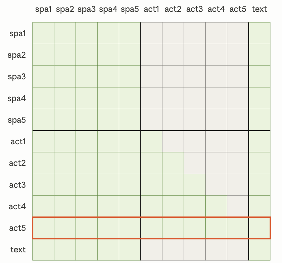
여기서 t=5라 생각하고 보면된다. (spa3= \(F_{spa,t-2}\) ) \(F_{spa}\)끼리는 서로 self-attention을 통해 시간에 따른 과거부터 현재 장면이 어떻게 변했는지를 학습한다. (양방향으로 봄)
\(F_{act}\)는 masked self-attention을 통해 \(F_{spa}\)로 얻은 장면 변화와 이전 action을 참고하여 현재 시점에서 어떤 행동을 해야하는지 학습한다. (autoregressive로 봄)

output

\(F_{tem}\)은 Transformer를 통과하면서 시간 문맥이 반영된 feature이다

Casual Transformer를 통과한 Teacher feature들은

F_{\text{tem}, t-4}^{T}, \ F_{\text{tem}, t-3}^{T}, \ F_{\text{tem}, t-2}^{T}, \ F_{\text{tem}, t-1}^{T}, \ F_{\text{tem}, t}^{T}

가 나오고 Student feature들은

F_{\text{tem}, t-4}^{S}, \ F_{\text{tem}, t-3}^{S}, \ F_{\text{tem}, t-2}^{S}, \ F_{\text{tem}, t-1}^{S}, \ F_{\text{tem}, t}^{S}

가 된다.

\(G_t\)는 \(F_{tem}\)를 통해 시간에 따라 어떻게 변하는지 계산한다.

그런데 데이터가 연속 시간이 아니라 프레임 단위로 끊겨 있으므로, 미분 대신 앞뒤 프레임 차이를 이용해 변화량을 근사한다.

\begin{align*} G_t^T &= \nabla_t F_{\text{tem}}^T \\ G_t^S &= \nabla_t F_{\text{tem}}^S \end{align*}

central difference G는 앞뒤 feature가 모두 있어야 하므로 양 끝에서는 계산하지 않는다. 예를들어 t=5라면

t-4   t-3   t-2   t-1   t
 X     O     O     O    X

G는 아래 3시점에서만 계산된다.

G_{t-3}, \ G_{t-2}, \ G_{t-1}

Teacher:

\begin{align*}G_{t-3}^T &= \frac{F_{\text{tem}, t-2}^T - F_{\text{tem}, t-4}^T}{2} \\G_{t-2}^T &= \frac{F_{\text{tem}, t-1}^T - F_{\text{tem}, t-3}^T}{2} \\G_{t-1}^T &= \frac{F_{\text{tem}, t}^T - F_{\text{tem}, t-2}^T}{2}\end{align*}

Student:

\begin{align*}G_{t-3}^S &= \frac{F_{\text{tem}, t-2}^S - F_{\text{tem}, t-4}^S}{2} \\G_{t-2}^S &= \frac{F_{\text{tem}, t-1}^S - F_{\text{tem}, t-3}^S}{2} \\G_{t-1}^S &= \frac{F_{\text{tem}, t}^S - F_{\text{tem}, t-2}^S}{2}\end{align*}

Temporal Dynamics Distillation의 목적은

G^T\approx G^S

Temporal Dynamics Distillation loss는 다음과 같다.

L_{TD} = \frac{1}{H - 2} \sum_{t = t_0 - H + 2}^{t_0 - 1} \left\| G_t^S - G_t^T \right\|_2^2

수식의 의미는 H−2개의 timestep에서 Student와 Teacher의 temporal gradient 차이를 평균낸다.

예를들어 H=5인경우 아래와 같다.

L_{TD} = \frac{1}{3} \left( \left\| G_{t-3}^S - G_{t-3}^T \right\|_2^2 + \left\| G_{t-2}^S - G_{t-2}^T \right\|_2^2 + \left\| G_{t-1}^S - G_{t-1}^T \right\|_2^2 \right)

Action Distribution Distillation

Input

Causal Transformer를 통과한 후 나온 Teacher의 action feature는 아래와 같고

\tilde{F}_{\text{act}, t-4}^{T}, \ \tilde{F}_{\text{act}, t-3}^{T}, \ \tilde{F}_{\text{act}, t-2}^{T}, \ \tilde{F}_{\text{act}, t-1}^{T}, \ \tilde{F}_{\text{act}, t}^{T}

Student는 아래와 같다.

\tilde{F}_{\text{act}, t-4}^{S}, \ \tilde{F}_{\text{act}, t-3}^{S}, \ \tilde{F}_{\text{act}, t-2}^{S}, \ \tilde{F}_{\text{act}, t-1}^{S}, \ \tilde{F}_{\text{act}, t}^{S}

Action distillation에서 사용되는 입력은 현재 시점의 액션만 사용된다.

\tilde{F}_{\text{act}, t}^{T},\;\tilde{F}_{\text{act}, t}^{S}

Output

Policy Head는 action feature를 받아서 action distribution을 출력한다.

Policy Head MLP로 구성되어 있으며 Teacher와 Student는 MLP의 가중치를 공유해서 사용하고 출력은 Gaussian action distribution의 parameter인 mean과 standard deviation을 출력한다.

\begin{align*}\tilde{F}_{\text{act}, t}^{T} &\rightarrow \text{Policy Head} \rightarrow \mu_t^T, \sigma_t^T \\\tilde{F}_{\text{act}, t}^{S} &\rightarrow \text{Policy Head} \rightarrow \mu_t^S, \sigma_t^S\end{align*}

따라서 다음과 같은 분포를 출력한다고 볼 수 있음으로

\begin{align*}A_t^T &= \mathcal{N}(\mu_t^T, \sigma_t^T) \\A_t^S &= \mathcal{N}(\mu_t^S, \sigma_t^S)\end{align*}

Action Distribution Distillation loss는 KL을 사용하여 계산하고 이 차이를 줄이도록 학습한다.

L_{AD} = KL(A_t^T \parallel A_t^S)

최종적으로는 이를 통해 Student가 이 distribution을 따라가면 RGB입력만 사용하더라도 Teacher의 3D-aware decision-making을 배울 수 있게된다.

Target actiont

teacher의 Target action *a는 아래와 같다.

L_{actor}= -\log\pi_{\theta}(a_t^*|o_t,g)

MonoLift: Learning 3D Manipulation Policies from Monocular RGB via Distillation

서론

목차

Problem Formulation

Spatial Representation Distillation

Input

Teacher branch

Student branch

Output

Temporal Dynamics Distillation

Input

Spatial Token

Learnable Acton Token

Language Token

Casual Transformer

output

Action Distribution Distillation

Input

Output

Target actiont

Comment