MobileNetV2 논문리뷰

서론

Mark Sandler, Andrew Howard, Menglong Zhu, Andrey Zhmoginov, Liang-Chieh Chen; Proceedings of the IEEE Conference on Computer Vision and Pattern Recognition (CVPR), 2018, pp. 4510-4520, MobileNetV2: Inverted Residuals and Linear Bottlenecks
위 논문에 대해서 리뷰하고 Depthwise Separable Convolution, Linear Bottlenecks, Inverted Residuals 에 대해서 자세히 살펴본다.
이 논문은 2018년도 4월에 Conference on Computer Vision and Pattern Recognition(CVPR)에서 발표되었다. CVPR은 컴퓨터 비전 분야의 가장 유명한 학술대화 중 하나다.

Abstract

1. we describe a new mobile architecture, mbox{MobileNetV2}, that improves the state of the art performance of mobile models on multiple tasks and benchmarks as well as across a spectrum of different model sizes.

본 논문은 여러 모델 크기에 따라서 성능을 측정하고 모바일 모델의 SOTA를 달성했다.

2. Is based on an inverted residual structure where the shortcut connections are between the thin bottleneck layers.

Bottleneck에 얇은 layer사이에 short connection을 적용한 도치된 Residual Structure를 갖는다.

3. The intermediate expansion layer uses lightweight depthwise convolutions to filter features as a source of non-linearity. Additionally, we find that it is important to remove non-linearities in the narrow layers in order to maintain representational power.

비선형성을 적용하여 feature를 filtering하기 위해 expansion layer를 사용하고 추가적으로 narrow layer에 representational power를 유지하기 위해 비선형성을 제거한다.

4. We measure our performance on mbox{ImageNet}~cite{Russakovsky:2015:ILS:2846547.2846559} classification, COCO object detection cite{COCO}, VOC image segmentation cite{PASCAL}.

classification인 경우 ImageNet Dataset
Object Detection인 경우 COCO Dataset
Segmentation인 경우 VOC Dataset

Introduction & Related Work

background Research

modern state of the art networks require high computational resources beyond the capabilities of many mobile and embedded applications.
현대 최신 모델들은 임베디드 장치가 수용할 수 있는 리소스 한계를 넘는 많은 연산량을 요구하는 자원을 필요로 한다.

Recent Research

recently, opened up a new direction of bringing optimization methods including genetic algorithms and reinforcement learning to architectural search.
However one drawback is that the resulting networks end up very complex.
최근에는 진화 알고리즘, 강화학습등을 통한 NAS기술을 도입해 최적화하는 기법이 적용되고 있다.
그러나 여전히 네트워크가 복잡하다는 단점이 있다.

Propose

we pursue the goal of developing better intuition about how neural networks operate and use that to guide the simplest possible network design.
우리는 신경망이 어떻게 동작하는지에 대해 더 나은 직관을 소개하고 가벼운 네트워크를 설계하는 방법에 대해 소개한다.

MobileNetV1

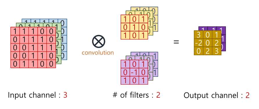
Convolution Operation
- input channel의 수 = filter channel의 수, filter의 갯수 = output channel 수
feature map 크기 계산방법 $O_h = floor(\frac{I_h - K_h+2P}{S}+1) \\Ow = floor(\frac{I_w - K_w+2P}{S}+1)$

floor: 소수점 발생시 소수점 이하는 버림

$I_h$ : 입력의 높이
$I_w$ : 입력의 너비
$K_h$ : 커널의 높이
$K_w$ : 커널의 너비
$S$ : 스트라이드
$O_h$ : feature map 높이
$O_w$ : feature map 너비

Padding = “same” : input shape과 output shape이 동일하도록 padding값이 들어감

padding=“valid”(padding=0): 3x3 kernel의 경우 input_shape이 (224, 224) –> (222, 222)로 출력됨
padding=“same”(padding=1): 3x3 kenrel의 경우 input_shape이 (224, 224) –> (224, 244)로 출력됨)

Convolution Operation

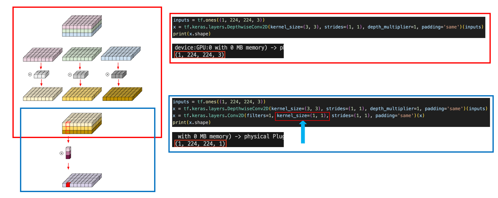
Depthwise Separable Convolution (depthwise conv + pointwise conv)

Depthwise Separable Convolution = Depthwise Conv + Pointwise Conv
Depthwise Conv : input feature map에 대해 output feature map의 채널수가 동일하다.

Computational Cost

$𝐷_𝐹$: height/width of feature map
$𝐷_𝐾$: height/width of filter
$M$: channel of Input Tensor
$N$ : channel of ouput Tensor(Number of filters)
Standard Convolutions computational cost
- $D_F\times D_F\times M \times D_K \times D_K \times N$
- $D_F\times D_F\times M $ 은 각 채널에 대한 계산 비용, $D_K \times D_k \times N$번 일어난다.
Depthwise Separable Convolution computational cost
- $D_F\times D_F\times M \times D_K \times D_K + D_F \times D_F \times M \times N$
Reduction in computations(Depth Conv / Standard Conv)
- $\frac{1}{N} + \frac{1}{D_K^2}$
$N$은 ouput_channel의 크기(=필터의 갯수)이고 $D_K$는 필터의 크기(shape) $N$이 $D_K$보다 일반적으로 훨씬 큰 값이므로 $\frac{1}{D_k^2}$ 값이 되어 $\frac{1}{D_k^2}$배 만큼 계산이 줄었다고 볼 수 있다.
이 때, $D_K$는 보통 3이므로 1/9배 정도 계산량이 감소함

Linear Bottlenecks (1)

Informally, for an input set of real images, we say that the set of layer activations forms a “manifold of interest”
Real Image를 input으로 받았을 때, Neural Network의 어떤 layer들을 통해 manifold를 형성한다.
It has been long assumed that manifolds of interest in neural networks could be embedded in low-dimensional subspaces.
manifold는 Neural Network에서 input의 feature들이 저차원의 subspace로 맵핑될 수 있다는 가정이 있다.
What is manifold?
- In neural networks, the concept of "manifold" refers to the idea that networks typically include an encoder component that compresses high-dimensional data into a lower-dimensional space. This process involves performing feature extraction.
- Neural Networks는 일반적으로 학습 과정에서 고차원의 데이터를 저차원으로 압축하는 encoder와 같은 역할을 하는데 이때 feature extraction을 하게된다.
- 고차원의 데이터가 저차원으로 압축되면서 특정 정보들을 잘 표현하는 저차원의 부분공간(subspace)로 맵핑되는데 이러한 공간을 manifold라고 한다.
We have highlighted two properties that are indicative of the requirement that the manifold of interest should lie in a low-dimensional subspace of the higher-dimensional activation space:
manifold는 고차원의 데이터를 저차원의 subspace로 맵핑이 가능하다는 것에 대해서 다음 두가지를 강조한다.
- If the manifold of interest remains non-zero volume after ReLU transformation, it corresponds to a linear transformation.
- 만약 ReLU를 통과 한 어떤 feature가 0보다 컸다면 ReLU의 특성상 identity Matrix를 곱한 것과 같아서 단순한 linear transformation하다고 볼 수 있다.
- ReLU is capable of preserving complete information about the input manifold, but only if the input manifold lies in a low-dimensional subspace of the input space.
- 네트워크를 거치면서 feature들이 저차원으로 매핑되는 연산이 계속되는데, 양수에 대해서는 ReLU는 그대로 전파하는 linear transformation이므로 manifold의 정보를 잘 보존하고 있다고 볼 수 있다.
assuming the manifold of interest is low-dimensional we can capture this by inserting linear bottleneck layers into the convolutional blocks.
- 즉, 저차원으로 매핑하는 bottleneck architecture를 만들 때, linear transformation역할을 하는 linear bottlenect layer를 만들어서 차원은 줄이되 manifold 상의 중요한 정보들은 그대로 유지해 보자는 것이 컨샙이다.

Linear Bottlenecks (2)

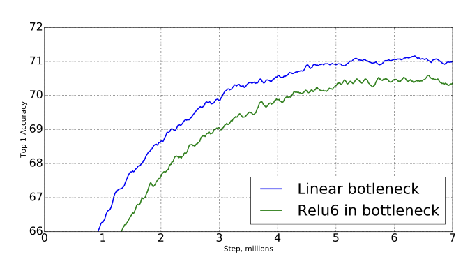
실제로 실험을 하였는데 bottlenect layer를 사용하였을 때 ReLU를 사용하면 오히려 성능이 떨어진다는 것을 확인했다.
However, the output of the projection layer does not have an activation function applied to it. Since this layer produces low-dimensional data, the authors of the paper found that using a non-linearity after this layer actually destroyed useful information.
projection layer는 activation function을 사용하지 않는데, 이 layer는 low-dimensional data를 가지고 있기 때문에 이후 비선형성 활성화함수를 사용하면 유용한 정보를 손실한다는 것을 발견했다.
아마 Relu가 0이상의 값에 대해서는 그대로 전파하지만 0이하의 값은 전부 0으로 고정시킴으로 정보손실이 잃어나 학습에 영향을 주는 것이 아닐까 추측한다.

Inverted Residuals

Inspired by the intuition that the bottlenecks actually contain all the necessary information, while an expansion layer acts merely as an implementation detail that accompanies a non-linear transformation of the tensor, we use shortcuts directly between the bottlenecks.
Expansion layer는 feature map의 non-linear transformation을 수행하고 Bottlenecks(빗금친부분)는 필요한 정보만 압축해 저장하고 있다라는 직관에 영감을 받아 skip connection을 사용하면 필요한 정보를 더 깊은 layer까지 잘 전달 할 것이라는 기대를 할 수 있다. 그리고 기존 Residual block구조에서 도치된 형태로사용함으로써 메모리 사용량을 줄일 수 있다.
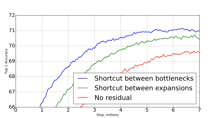
(오른쪽 이미지 표) narrow layer에 residual connection을 적용한 것, residual connection을 expansion layer에 적용한 것, residual connection을 아이에 적용하지 않은 것에 대한 성능차이를 보여주는 표이다.

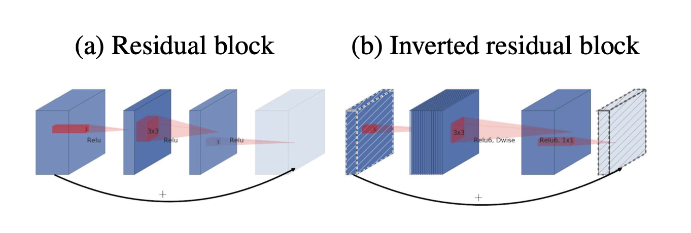
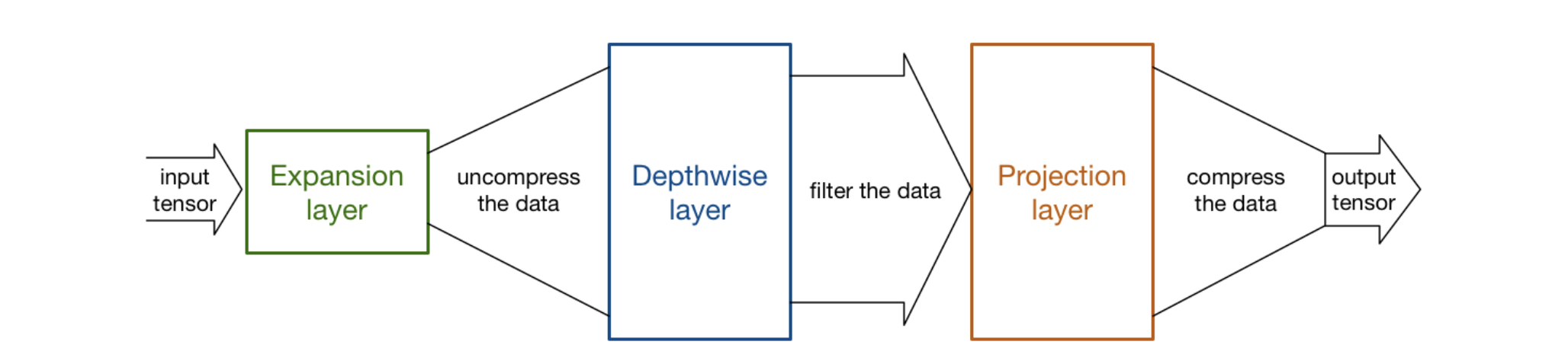
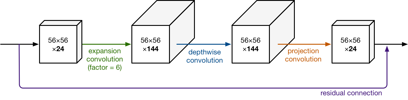
feature map이 들어오면 1x1 conv를 통해 dimension을 expand시키고 feature를 filtering하기 위한 3x3 depthwise conv연산을 합니다. 마지막에는 1x1 conv을 통해 skip conntection과 합쳐지기 위해 원래의 dimension으로 복원하게 된다.

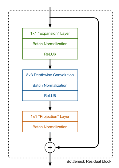
Bottleneck Residual Blocks

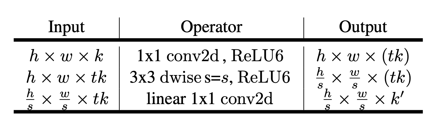
The basic building block is a bottleneck depth-separable convolution with residuals.

입력이 Narrow상태로 들어오면
1x1conv(expansion layer)를 통해 채널을 키운다.
BatchNorm -> ReLU6
3x3 depthwise conv를 통해 feature filtering
BatchNorm -> ReLU6
1x1conv를 사용해 채널 수를 다시 복원(줄인다)
skip connection을 사용한다.

expansion factor t를 사용하여 filter에 곱해서 채널을 확장시킵니다. 이 논문에서는 t를 6으로 사용하고 있으며 논문에서는 5~10정도를 사용하는것을 추천한다.

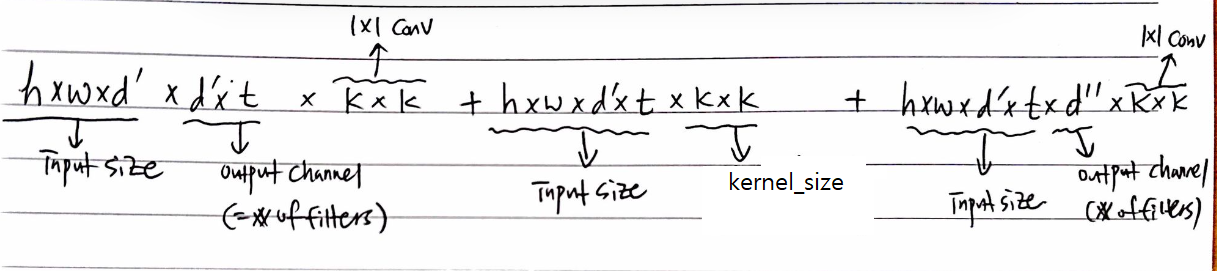
Number of Operations(Multiply-add)

Input size: $h \times w$
Expansion factor: $t$
Kernel size: $k$
Input channels: $d'$
Output channels: $d''$
The total number of multiply add required is

h \times w \times d' \times d' \times t + \\ h \times w \times d' \times t \times k \times k + \\ h\times w\times d'\times t \times d'' \\= h\times w\times d'\times t(d'+k^2+d'')

The Architecure of MobileNetV2

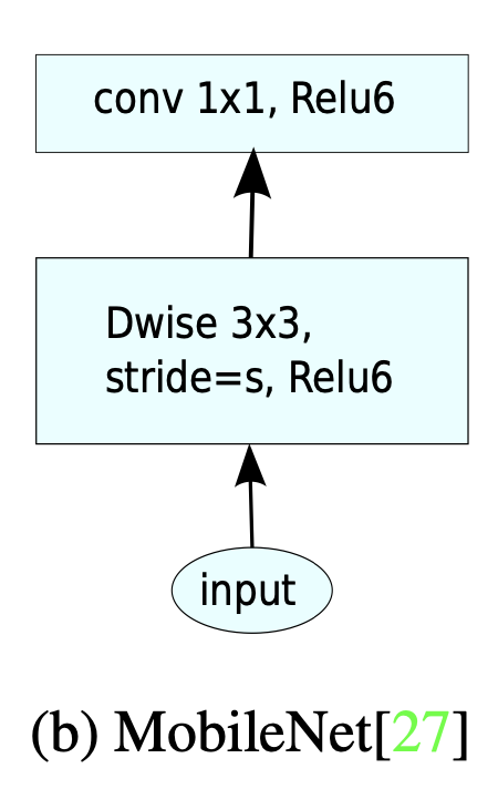
MobileNetV1

MobileNetV1에서의 block은 크게 2개의 layer로 구성되어 있다.
첫번째 layer인 depthwise convolution은 각 Input channel에 single convolution filter를 적용하여 네트워크 경량화를 하는 작업이였다.
두번째 layer는 pointwise convolution인 1x1 convolution에서는 depthwise convolution의 결과를 pointwise convolution을 통하여 다음 layer의 Input으로 합쳐주는 역할을 한다.
Activation function으로 ReLU6를 사용하여 block을 구성하였다.
참고로 ReLU6는 min(max(x, 0), 6) 식을 따르고 음수는 0으로 6이상의 값은 6으로 수렴시킨다.

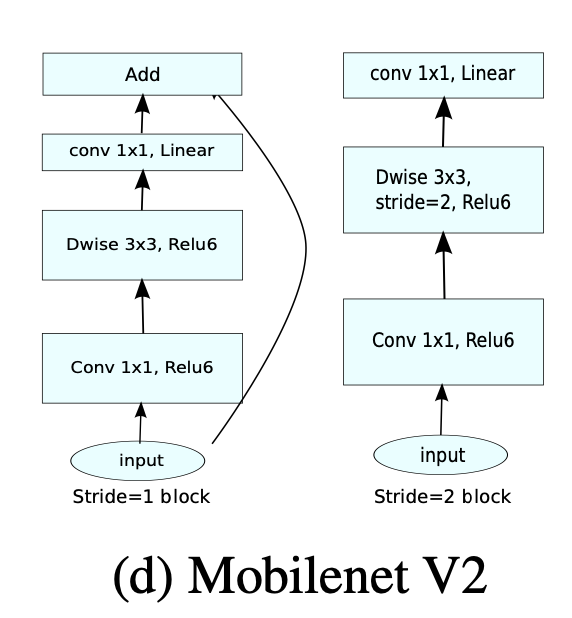
MobileNetV2

MobileNetV2에는 크게 2가지 종류의 block이 있다.
2가지 종류의 block은 3개의 layer를 가지고 있습니다.
두 종류의 block 모두 첫 번째 layer는 1x1convolution + ReLU6 입니다.
stride = 1 경우
- depthwise convolution, stride=1로 설정한다.
stride = 2 경우
- depthwise convolution, stride=2로 설정되어 downsizing 된다.
세번째 layer에서는 pointwise(1x1) convolution이 적용된다.
단, 여기서는 activation function이 없다. 즉, non-linearity를 적용하지 않은 셈이다.
stride가 2가 적용된 block에는 skip connection이 없다.
stride 2를 적용하면 feature의 크기가 반으로 줄어들게 되므로 skip connection 또한 줄어든 크기에 맞게 맞춰져야 하는 문제가 있어서 skip connection은 적용하지 않은 것으로 추정된다.

MobileNetV2 - Not applied Residual connection

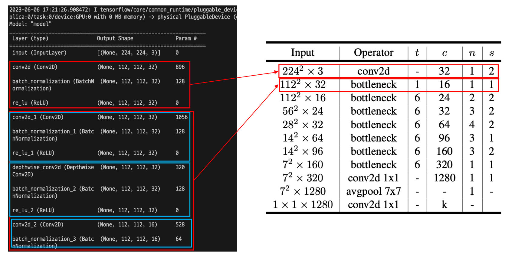
처음 빨간 네모박스는 일반 Conv2d를 진행
bottleneck부분에서는 expansion–> Depthwise –> projection 순으로 진행
residual connection은 stride=1이고 input, output의 shape이 같은 경우에만 해주는데 해당 네모박스 부분은 다르기 때문에 하지 않는다.
- (None, 112, 112, 3) ≠ (None, 112, 112, 64)

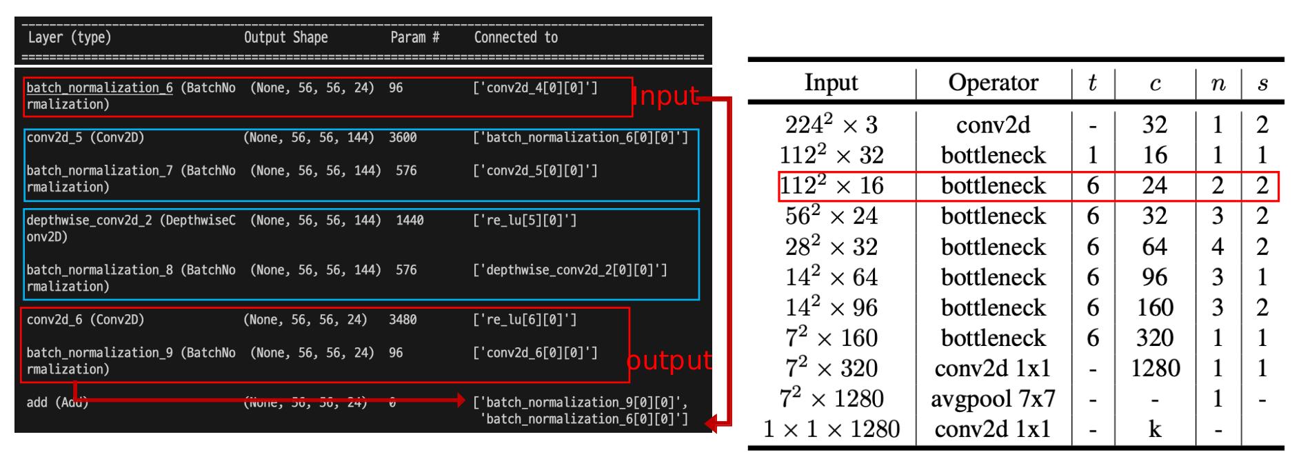
MobileNetV2 - Applied Residual connection

해당 부분은 residual connection을 하는 레이어인데, s=2인데도 불구하고 residual connection이 존재하는 이유는 [t=6, c=24, n=2, s=2] n=1일때는 s=2로 가져가지만 n=2일때는 s=1로 코드상에 설정되어 있다.

The Max Number of Channels/Memory(KB)

Our primary network (width multiplier 1, 224 × 224), has a computational cost of 300 million multiply-adds and uses 3.4 million parameters.
기본 network에서는 width multiplier가 1이고 이미지 크기는 224, 224로 한다.
이렇게 설정했을 경우 3억(300million)의 계산량(multiply-adds) and 340만개(3.4 million)의 parameter를 사용한다.
Resolution Multiplier는 Input이미지를 일정한 비율로 줄인다.
width multiplier는 layer의 채널수를 일정 비율로 줄이는 역할을 한다. 기본이 1이며 만약 0.5인경우 절반으로 줄인다.(0~1 사이의 실수로 설정된다)

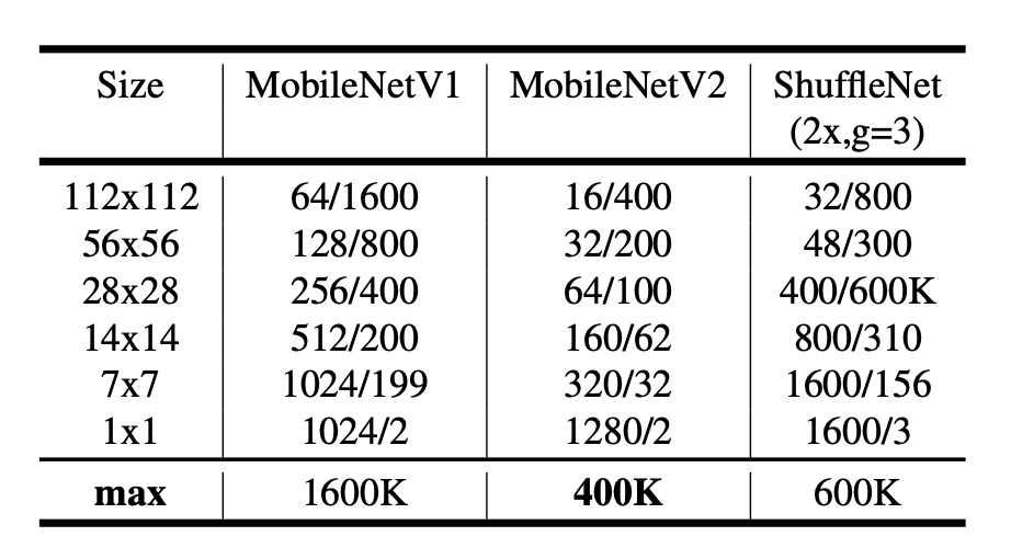
(이미지 - 표)

위 테이블에서는 각 input_size에 따른 mobilenet, mobilenet v2, shufflenet에 대한 채널의 수/메모리(Kb 단위)의 최대 크기를 기록하였다.
논문에서는 400kilobyte mobilenet v2의 크기가 가장 작다고 설명하고 있다.

Experiments - ImageNet Classification

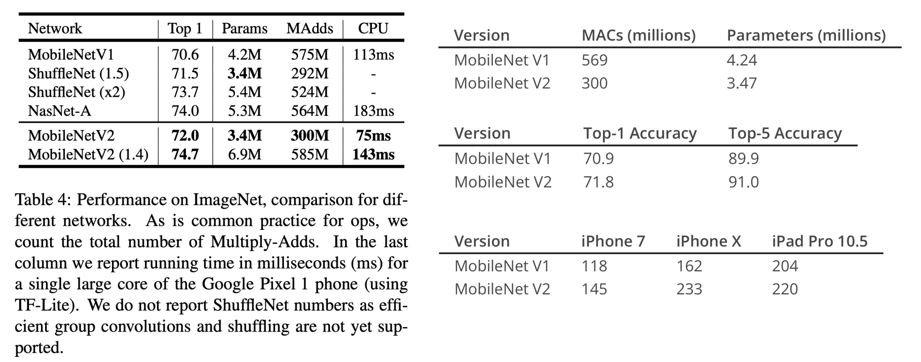
왼쪽 표는 Google Pixel 1에서 TF-Lite로 변환해 시간과 정확도에 대해서 측정한 지표이다.
MBV2
- parameter: 340만개(=3.4M)
- MAdds: 3억개(=300M)
오른쪽 첫번째 표는 어떤 웹사이트에서 발견건데 학습에 필요한 parameter와 계산량의 관점에서 본 표이다.
224x224 RGB single Image에 대한 MBV1, MBV2에 대한 연산량과 파라미터 수를 보여줍니다.
오른쪽 두번째 표는 ImageNet classification dataset으로 측정된 정확도이다.
오른쪽 세번째 표는 모바일 기기의 CPU+GPU를 활용해 측정한 표이다(단위 224x224 image를 연속적으로 넣었을 때의 Maximum FPS)

Experiments - Object Detection(SSDLite)

We replace all the regular convolutions with depthwise separable convolutions (depthwise followed by 1 × 1 projection) in SSD prediction layers.

SSD Network의 bbox정보를 얻는(prediction layer쪽의) 3x3convolution layer를 전부 depthwise seperable convolution으로 교체하여 연산량을 줄였다. 결과 또한 연산을 줄였는데도 성능이 비슷하다.

Parameter

SSD(기본)

Params: 1480만개(=14.8M)
MAdds: 12억개(1.2B)

SSD Lite(Conv → Depthwise Separable Conv)

Params: 210만개(=2.1M)
MAdds: 3억5천만개(=0.35B)

Results

MNetV2+SSDLite

Params: 430만개(=4.3M)
MAdds: 8억개(=0.8B)

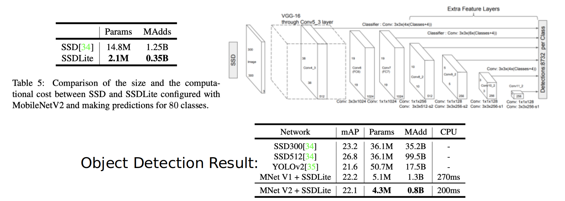
SSD300 : 300x300 Input Size
SSD512 : 500x500 Input Size
MNetV1+SSDLite : MobileNetv2를 backbone으로 한 SSD Lite

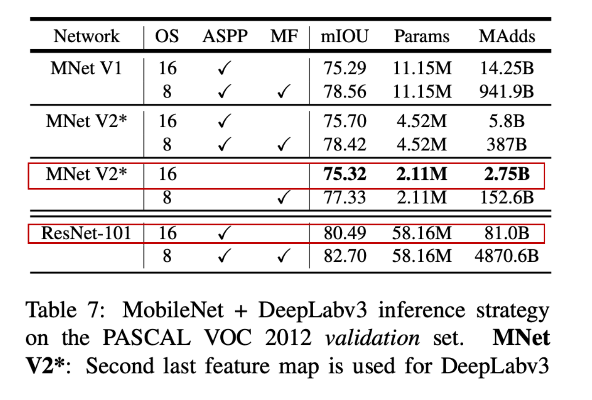
Experiments - Segmentation Results

MobileNetV2

Parameter: 211만개(2.11million == 2,110,000)
MAdds: 27억5000만개(2.75billion == 2,750,000,000)

ResNet-101

Parameter: 5816만개(58.11million == 58,160,000)
MAdds: 810억개(81.0billion == 81,000,000,000)

OS는 Output Stride의 약자로 해상도 비율을 나타낸다.

예를 들어, 네트워크가 Input Stride 1로 시작해서 여러 Convolutional Layer를 통과하며, Stride 2인 Max Pooling Layer를 두 번 통과했다면, 최종 Output Stride는 4가 됩니다. 이는 출력 특성 맵의 한 픽셀이 입력 이미지의 4x4 픽셀 구간에 해당한다는 의미다.
Output Stride가 크면 모델의 계산 비용은 줄어들지만, 해상도가 떨어져 세부 정보를 놓칠 수 있다.
반면 Output Stride가 작으면 해상도가 향상되지만 계산 비용이 증가한다.
이러한 특성 때문에 Output Stride는 특히 이미지 분할(Image Segmentation) 같은 작업에서 중요한 개념이 된다.
MF는 "Multiply-Accumulate Operation (MACs)" 혹은 "Million Flops"의 약자
mIOU는 "mean Intersection over Union"을 나타내며, 세그멘테이션 성능을 평가하는 주요 지표다

[reference]

https://arxiv.org/abs/1801.04381

https://gaussian37.github.io/dl-concept-mobilenet_v2/

https://machinethink.net/blog/mobilenet-v2/

MobileNetV2 논문리뷰

서론

목차

Abstract

Introduction & Related Work

background Research

Recent Research

Propose

Related Paper

MobileNetV1

Convolution Operation

Depthwise Separable Convolution (depthwise conv + pointwise conv)

Computational Cost

Linear Bottlenecks (1)

Linear Bottlenecks (2)

Inverted Residuals

Bottleneck Residual Blocks

Number of Operations(Multiply-add)

The Architecure of MobileNetV2

MobileNetV1

MobileNetV2

MobileNetV2 - Not applied Residual connection

MobileNetV2 - Applied Residual connection

The Max Number of Channels/Memory(KB)

Experiments - ImageNet Classification

Experiments - Object Detection(SSDLite)

Parameter

Results

Experiments - Segmentation Results

Comment