DRÆM

서론

Vitjan Zavrtanik, Matej Kristan, Danijel Skočaj; Proceedings of the IEEE Conference on Computer Vision and Pattern Recognition (CVPR), 2021, pp. 1-10. DRÆM – A Discriminatively Trained Reconstruction Embedding for Surface Anomaly Detection.
논문 리뷰: DRÆM – A discriminatively trained reconstruction embedding for surface anomaly detection 논문 리뷰
https://arxiv.org/pdf/2108.07610.pdf

Introduction & Related Work

background Research

Recent surface anomaly detection methods rely on generative models to accurately reconstruct the normal areas and to fail on anomalies.

최근 surface anomaly detection방법들이 generative model을 활용하여 정상적인 이미지에 대해서는 정확하게 reconstruction하고 비정상적인 이미지에서는 실패하는 방식으로 네트워크가 설계되었다.

Recent Research

Reconstructive methods, such as Autoencoders [5, 1, 2, 26] and GANs [24, 23], have been extensively explored since they enable learning of a powerful reconstruction subspace, using only anomaly-free images.

AutoEncoder와 GANs와 같은 Reconstructive 방법은 정상적인 이미지만을 가지고 강력한 reconstruction subspace(부분공간)을 학습할 수 있음으로 광범위하게 탐구되었다.

These methods are trained only on anomaly-free images, and often require hand-crafted post-processing steps to localize the anoma- lies, which prohibits optimizing the feature extraction for maximal detection capability.

이러한 방법은 이상치가 없는 이미지(anomaly-free images)에 대해서만 학습해야 하고 이상치(anomaly)가 어디에 위치하는지 식별하기 위해 서는 사람이 손수 후처리 단계를 요구한다. 그러나 손수 후처리 과정이 모델의 학습 과정에 포함되어 있지 않기 때문에 이상치의 위치를 감지에 필요한 중요한 feature extraction을 최적화하지 못하게 된다.

Significant effort has thus been recently invested in designing robust surface anomaly detection methods that preferably require minimal supervision from manual annotation.

그래서 최근에는 최소한의 라벨링으로 Robust한 surface anomaly detection 설계에 상당한 노력이 이뤄진다.

Propose

In addition to reconstructive approach, we cast surface anomaly detection primarily as a discriminative problem and propose a discrimi- natively trained reconstruction anomaly embedding model (DRÆM).

우리는 앞서 설명한 reconstructive 접근 방식 뿐만 아니라 discriminative 접근 방식도 사용하여 surface anomaly detection을 다루는 DRÆM에 대해 소개한다.

The method enables direct anomaly localization without the need for additional complicated post-processing of the network output and can be trained using simple and general anomaly simulations.

이 방법을 사용하면 네트워크의 output을 가지고 복잡한 후처리 작업 없이 이상치가 어디에 위치하는지 식별할 수 있으며 이 방법을 통해 쉽게 이상치를 탐지해 낼 수 있으며 더 좋은 성능을 보인다.

Abstract

Visual surface anomaly detection aims to detect local image regions that significantly deviate from normal appearance.

Visual surface anomaly detection은 이미지의 일부 local한 부분이 정상적인 외형에서 벗어난 경우를 감지하는 것을 목표로한다.

Recent surface anomaly detection methods rely on generative models to accurately reconstruct the normal areas and to fail on anomalies.

최근 surface anomaly detection방법들이 generative model을 활용하여 정상적인 이미지에 대해서는 정확하게 reconstruction하고 비정상적인 이미지에서는 실패하도록 설계되었다.

이러한 방법은 이상치가 없는 이미지에 대해서만 학습해야 하며 이상치가 어디에 위치하는지 식별하기 위해 서는 사람이 손수 후처리 단계를 요구한다. 그러나 손수 후처리 과정이 모델의 학습 과정에 포함되어 있지 않기 때문에 이상치의 위치를 감지에 필요한 중요한 feature extraction을 최적화하지 못하게 된다.

우리는 앞서 설명한 reconstructive 접근 방식 뿐만 아니라 discriminative 접근 방식도 사용하여 surface anomaly detection을 다루는 DRÆM에 대해 소개한다.
discriminative 접근 방식은 이상치와 정상치 사이의 차이를 학습하여 두 클래스를 구분한다.

The proposed method learns a joint representation of an anomalous image and its anomaly-free reconstruction, while simultaneously learning a decision boundary between normal and anomalous examples.

본 논문은 데이터의 reconstructive을 학습하면서 동시에 reconstruction가 생성한 정상 데이터와 이상치 데이터를 같이 학습하여 이상치를 감지하게 된다.
이를 통해 이상치 감지의 정확성을 향상시키려는 것이다.

The method enables direct anomaly localization without the need for additional complicated post-processing of the network output and can be trained using simple and general anomaly simulations.

이 방법을 사용하면 네트워크의 output을 가지고 복잡한 후처리 작업 없이 이상치가 어디에 위치하는지 식별할 수 있으며 이 방법을 통해 쉽게 이상치를 탐지해 낼 수 있다.
On the challenging MVTec anomaly detection dataset, DRÆM outperforms the current state-of-the- art unsupervised methods by a large margin and even delivers detection performance close to the fully-supervised methods on the widely used DAGM surface-defect detection dataset, while substantially outperforming them in localization accuracy.
DRÆM은 까다로운 anomaly detection dataset인 MVTec에서 비지도 학습으로 우수한 성적을 보였고 surface-defect detection dataset DAGM에서 지도학습으로 좋은 성능을 보였다.

Introduction

Surface anomaly detection addresses localization of image regions that deviate from a normal appearance (Figure 1).

Surface anomaly detection은 이미지내에서 위치한 비정상적인 부분을 감지한다.

A closely related general anomaly detection problem considers anomalies as entire images that significantly differ from the non-anomalous training set images.

일반적인 anomaly detection problem은 이미지 전체를 보고 비정상 이미지로 판단한다. 이는 학습에 사용된 정상 이미지와 크게 다른 경우의 이미지를 고려한다.
쉽게 말해, 이미지를 전체적으로 보았을 때 학습 데이터 셋의 '정상' 이미지와 얼마나 다른지를 기반으로 그 이미지가 비정상이미지인지 아닌지를 판단하는데 이 방법은 이상치가 이미지 내의 부분 또는 세부적인 것에 국한되지 않고, 전체 이미지 수준에서 판단된다는 것이다.

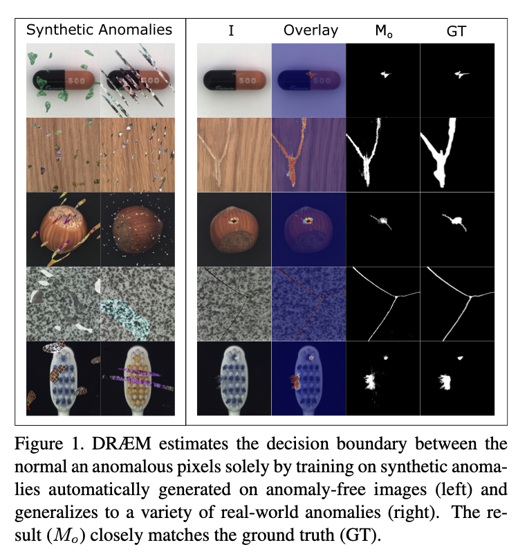
In contrast, in surface anomaly detection problems, the anomalies occupy only a small fraction of image pixels and are typically close to the training set distribution. This is a particularly challenging task, which is common in quality control and surface defect localization applications.

반면에, surface anomaly detection는 이미지의 비정상적인 부분을 작은 영역의 픽셀로 나타내며 이러한 비정상 이미지는 일반적으로 학습 데이터의 분포에 가까운 아주 유사한 이미지 라는 것이다. 이는 특히 품질 관리 및 표면의 결함을 찾아내는 어려운 작업이다.

In practice, anomaly appearances may significantly vary, and in applications like quality control, images with anomalies present are rare and manual annotation may be overly time consuming.

실제로, anomaly 부분은 매우 다양하게 나타날수 있으며, 품질 관리와 같은 측면에서 볼 때 결함이 있는 이미지는 상대적으로 결함이 없는 이미지 보다 데이터 수가 적어 라벨링 작업에서 매우 많은 시간이 소모될 수 있다.

This leads to highly imbalanced training sets, often containing only anomaly-free images.

이러한 이유로 training dataset은 주로 정상적인 이미지만을 포함하게 됨으로 데이터 분포가 매우 불균형하게 된다.

Significant effort has thus been recently invested in designing robust surface anomaly detection methods that preferably require minimal supervision from manual annotation.

그래서 최근에는 최소한의 라벨링으로 Robust한 surface anomaly detection 설계에 상당한 노력이 이뤄진다.

AutoEncoder와 GANs와 같은 Reconstructive 방법은 정상적인 이미지만을 가지고 강력한 reconstruction subspace(부분공간)을 학습할 수 있음으로 광범위하게 탐구되었다.

Relying on poor reconstruction capability of anomalous regions, not observed in training, the anomalies can then be detected by thresholding the difference between the input image and its construction.

anomaly한 영역은 training에서 단계에서 학습되지 않기 때문에, 입력 이미지와 그 reconstruction 사이의 차이를 임계값으로 설정함으로써 이상치를 감지할 수 있다.

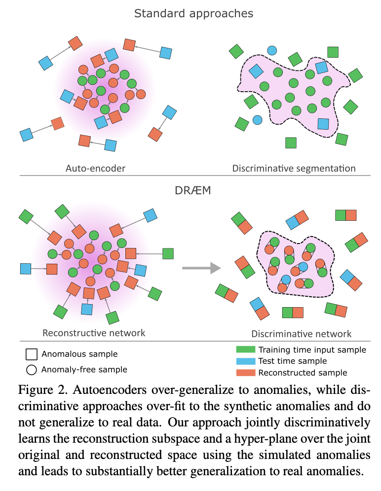
However, determining the presence of anomalies that are not substantially different from normal appearance remains challenging, since these are often well reconstructed, as depicted in Figure 2, top-left.

그러나 세부적인 anomlay들은 종종 잘 복원되기 때문에, 이를 감지하는 것이 어렵다. 이는 논문의 그림 2, 왼쪽 상단에 있다.

Recent improvements thus consider the difference between deep features extracted from a general-purpose network and a network specialized for anomaly-free images [4].

최근 위 문제를 개선한 사항으로는 general-purpose의 네트워크에서 추출된 특징들과 이상치가 없는 이미지들에 특화해 학습환 네트워크 사이의 차이를 고려한다는 것이다.
예를 들어, 일반적인 목적(general-purpose)의 네트워크는 이미지의 다양한 특징을 인식하고 이해하는 데 중점을 두는 반면, 이상치가 없는 이미지들을 위한 전문 네트워크(specialized network)는 이상치가 없는 이미지의 특정 특징에 초점을 맞추고 있을 수 있다.
따라서, 이 두 네트워크에서 추출된 깊은 특징들 사이의 차이를 고려함으로써, 이상치 감지의 정확성을 향상시킬 수 있다.

Discrimination can also be formulated as a deviation from a dense clustering of non-anomalous textures within the deep subspace [22, 7], as forming such a compact subspace prevents anomalies from being mapped close to anomaly-free samples.

네트워크의 어떤 고차원 공간에서 정상적인 이미지의 특성들은 서로 밀집된 형태로 있게 되는데 Discrimination은 이러한 정상이미지의 클러스터에 비정상 이미지가 맵핑되는 것을 방지한다. 따라서 비정상 이미지는 정상 이미지의 클러스터에서 벗어나 있을 가능성이 높으며 이러한 둘의 차이를 deviation(편차)로 표현할 수 있다.
편차로서 표현될 수 있다는 것을 설명하고 있습니다. 이러한 컴팩트한 부분 공간을 형성함으로써, 이상치가 이상치가 없는 샘플에 가깝게 매핑되는 것을 방지할 수 있습니다.
예를 들어, 우리가 얼굴 이미지를 처리하는 딥 러닝 모델을 가지고 있다고 가정해보자. 이 모델의 깊은 부분 공간에서, 정상적인 얼굴 텍스처들은 밀집된 클러스터를 형성할 것이다. 그러나 비정상적인 얼굴 이미지 (예를 들어, 얼굴에 큰 흉터가 있는 이미지)는 이 밀집된 클러스터에서 벗어나 있을 것임으로 이상치 감지는 이 밀집된 클러스터에서의 편차를 찾는 것으로 표현될 수 있다는 것이다.

A common drawback of the generative methods is that they only learn the model from anomaly-free data, and are not explicitly optimized for discriminative anomaly detection, since positive examples (i.e., anomalies) are not available at training time.

generative methods의 일반적인 단점은 정상 이미지만을 학습으로 사용하고 비정상 이미지를 학습에 사용하지 않기 때문에 discriminative anomaly detection의 비정상 이미지를 탐지하는 것에 최적화되기 어렵다.

Synthetic anomalies could be considered to train discriminative segmentation methods [8, 21], but this leads to over-fitting to synthetic appearances and results in a learned decision boundary that generalizes poorly to real anomalies (Figure 2, top-right).

합성된 비정상 이미지(인위적으로 생성한 이상치, Synthetic anomalies)를 사용하여 discriminative segmentation 방법을 사용해 훈련시킬 수 있지만, 이는 합성된 비정상 이미지에 대한 over-fitting을 초래하고, 실제 비정상 이미지에 대해서는 잘 일반화되지 않는 decision boundary를 생성할 수 있다.(그림 2, 오른쪽 상단)

We hypothesize that over-fitting can be substantially reduced by training a discriminative model over the joint, reconstructed and original, appearance along with the reconstruction subspace.

over-fitting을 크게 줄일 수 있는 가설은 본 논문에서 제안하는데, Discriminative 네트워크를 학습시킬 때 reconstructed된 이미지와 원본 이미지를 합치는 방법을 사용하면 이상치가 있는 부분과 없는 부분의 차이가 명확히 드러날 것이고, 이미지를 복원하는 과정에서 만들어내는 고차원 특징 공간인 reconstruction subspace에는 이미지의 특징이 잘 표현되어 있으므로 두 가지 정보를 사용하여 학습시키겠다는 것이다.

This way the model does not overfit to resynthetic appearance, but rather learns a local-appearance-conditioned distance function between the original and reconstructed anomaly appearance, which generalizes well over a range of real anomalies (see Figure 2, bottom).

이 방법을 통해 모델이 resynthetic appearance(합성된 비정상 이미지에)에 overfit되지 않고, local-appearance-conditioned distance function을 사용해 원본 이미지와 reconstructed된 이미지간의 차이를 측정하겠다는 것이다. 이 차이를 측정하는 거리 함수를 학습함으로써, 모델은 다양한 실제 이상치에 대해 잘 일반화할 수 있을 것이다.

To validate our hypothesis, we propose, as our main contribution, a new deep surface anomaly detection network, discriminatively trained in an end-to-end manner on synthetically generated just-out-of-distribution patterns, which do not have to faithfully represent the target-domain anomalies.

가설을 검증하기 위해, 본 논문에서는 인위적으로(합성) 생성된 학습 데이터의 분포에서 약간 바깥에 있는 분포 데이터들의 패턴들에 대해 end-to-end 방식을 사용하고 판별적 학습(discriminative learning)을 통해 새로운 surface anomaly detection network를 제안한다.
쉽게 말해 학습할 때 정상적인 이미지를 판별하기 위해 기존의 학습 데이터(정상이미지)도 보고 학습 데이터에서 약간 벗어난 데이터(just-out-of-distribution) 즉, 정상적인 분포에서 약간 벗어난 패턴을 학습에 사용하여 다양한 상황을 학습하도록 만든다. 따라서 실제 Target Domain에 해당하는 비정상적인 이미지를 정확하게 반영하지 않아도 어느정도 잘 감지할 수 있다는 것이 컨샙이다.

The network is composed of a reconstructive subnetwork, followed by a discriminative subnetwork (Figure 3).

이 제안하는 네트워크는 reconstructive subnetwork가 앞단에, discriminative subnetwork가 뒷단에 있다.

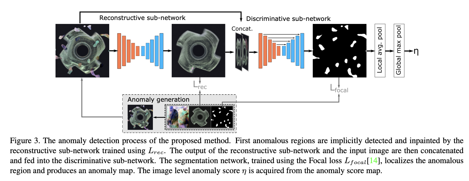
The reconstructive subnetwork is trained to learn anomaly-free reconstruction, while the discriminative subnetwork learns a discriminative model over the joint appearance of the original and reconstructed images, producing a high-fidelity per-pixel anomaly detection map (Figure 1).

reconstructive subnetwork는 정상이미지(anomaly-free)를 reconstruction하도록 학습하고 discriminative subnetwork는 input이미지(original image)와 reconstructive subnetwork를 통해 나온 reconstruction image 사이의 차이를 학습하여 이상치를 판별한다. 그리고 두 네트워크가 연결되어 동작하면서 고해상도 픽셀 별 anomaly detection map을 출력한다.

In contrast to related approaches that learn surrogate generative tasks, the proposed model is trained discriminatively, yet does not require the synthetic anomaly appearances to closely match the anomalies at test time and out-performs the recent, more complex, state-of-the-art methods by a large margin

이상치 검출(anomaly detection)을 위해 생성 모델을 사용하는 기존의 방법과는 달리(실제 비정상 이미지가 아닌 인위적으로 생성한 합성 비정상 이미지), 제안된 모델은 생성 모델이 아닌 판별 모델로서 학습된다(비정상 이미지와 정상이미지를 구별하는 것) 이 모델을 훈련시키기 위해 인위적으로 생성된 비정상 이미지(합성 비정상 이미지)는 실제 이상치와 완벽히 일치하지 않아도 이 모델은 잘 작동한다. 왜냐하면 이상치의 일반적인 특성만 학습하면 되기 때문이다. 따라서 학습 데이터가 실제 이상치와 완벽히 일치하지 않지만, 이 방법은 최근에 나온 더 복잡한 방법들보다 훨씬 더 좋은 성능을 보여준다.

Related work

Many surface anomaly detection methods focus on image reconstruction and detect anomalies based on image reconstruction error [1, 2, 5, 24, 23, 26, 31].

대부분의 surface anomaly detection방법은 이미지 생성에 해당하는 reconstruction에 초점을 맞추고 reconstruction error를 통해 anomaly detection을 한다.

Auto-encoders are commonly used for image reconstruction. In [1, 2, 26] auto-encoders are trained with adversarial losses.

Auto-Encoder는 주로 이미지 reconstruction(생성)에 해당되는데, 이는 adversarial(적대적) loss로 훈련된다.(적대적 생성 신경망은 Generator(생성자)와 Discriminator(식별자)가 서로 경쟁(Adversarial)하며 데이터를 생성(Generative)하는 모델(Network)을 뜻한다.)

The anomaly score of the image is then based on the image reconstruction quality or in the case of adversarially trained auto-encoders, the discriminator output.

이미지의 anomaly score는 reconstruction 이미지의 quality 또는 adversarially trained(적대적으로 훈련된) auto-encoders의 경우 discriminator의 출력을 기반으로 한다.

In [24, 23] a GAN [13] is trained to generate images that fit the training distribution.

GAN은 훈련 데이터셋의 분포를 학습해 훈련 데이터셋과 일치하도록 이미지를 생성해 낸다.

In [23] an encoder network is additionally trained that finds the latent representation of the input image that minimizes the reconstruction loss when used as the input by the pretrained generator.

encoder 네트워크를 추가로 학습시켜 encoder가 input 이미지의 latent space(latent representation)을 찾아내는데 reconstruction loss를 최소화 하기 위해 input 이미지의 latent space를 학습한다.

The anomaly score is then based on the reconstruction quality and the discriminator output.

anomaly score는 reconstruction quality와 discriminator의 출력에 기반한다.

In [29] an interpolation auto-encoder is trained to learn a dense representation space of in distribution samples.

Interpolation auto-encoder는 sample 분포 대한 representation space를 학습한다.

The anomaly score is then based on a discriminator, trained to estimate the distance between the input-input and input output joint distributions, however the approach to surface anomaly detection remains generative as the discriminator evaluates the reconstruction quality. (정통적인 auto encoder 방법)

Anomaly score는 입력-입력 및 입력-출력 결합 분포 간의 거리를 추정하도록 훈련된 판별자를 기반으로 한다. 그러나 (기존) surface anomaly detection 방식은 reconstruction quality를 평가하는 discriminator로 인해 여전히 generative하다.
쉽게 설명하면 Auto-encoder의 입력과 출력에 대한 joint distribution의 거리를 측정하는 discriminator가 있는데 이 joint distribution는 입력 이미지와 입력 이미지로 부터 생성한 출력 이미지(reconstruction Image) 사이의 관계를 나타낸다.
discriminator는 입력 이미지와 reconstruction Image 사이의 거리를 측정하는 역할을 하며 이 거리는 Anomaly score를 계산하는데 사용된다.
만약 reconstruction Image가 원래 이미지와 매우 다르다면, 이는 Input Image가 비정상 이미지라고 생각할 수 있으므로 이 거리(또는 차이)가 크면 Anomaly score도 높게 책정된다.
따라서 이 방법은 discriminator가 reconstruction된 이미지의 quality를 평가한다는 점에서 generative한 anomaly detection이라고 말한다.
왜냐하면 네트워크가 입력 이미지를 reconstruction하고, 그 reconstruction의 quality를 판별하는(discriminative) 방식을 통해 anomaly detection(이상치를 탐지)하기 때문이다.

Instead of the commonly used image space reconstruction, the reconstruction of pretrained network features can also be used for surface anomaly detection [4, 25].

일반적으로 사용되는 image space reconstruction 대신에, pretrained network(decoder) 네트워크를 사용해 reconstruction하는 방법도 surface anomaly detection에 사용될 수 있다.

Anomalies are detected based on the assumption that features of a pre-trained network will not be faithfully reconstructued by another network trained only on anomaly-free images.

이상치는 정상 이미지에 대해서만 훈련된 네트워크(encoder)에 의해 pre-trained 네트워크(decoder)가 특징을 제대로 추출하지 못하기 때문에 이미지를 잘 reconstructued되지 않을 것이라는 가정을 기반으로 탐지한다.

Alternatively [20, 11] propose surface anomaly detection as identifying significant deviations from a Gaussian fitted to construction.

또는 정상적인 데이터의 분포를 가우시안 분포에 맞춰 학습하고, 이 분포에서 크게 벗어나는 데이터를 이상치로 판단하는 방식이다.

However, determining the presence of anomalies that are not substantially different from normal appearance remains challenging, since these are often well recon- structed, as depicted in Figure 2, top-left.

그러나, 정상 이미지의 모습과 크게 다르지 않은 비정상 이미지를 파악하는 것은 여전히 도전적인 작업이다. 왜냐하면 이러한 이상치들은 종종 잘 재구성되기 때문이다.

We hypothesize that over-fitting can be substantially reduced by training a discriminative model over the joint, reconstructed and original, appearance along with the reconstruction subspace.

reconstructed된 이미지와 원래 이미지를 함께 사용하여 훈련시킴으로써 over-fitting 문제를 해결할 수 있다는 가설을 세웠다.

This way the model does not overfit to anomaly-free features of a pre-trained network.

이 방식은 모델이 pre-trained된 네트워크(decoder)가 정상적인 이미지에 대해 over-fitting되지 않게 된다.

This requires a unimodal distribution of the anomaly-free visual features which is problematic on diverse datasets.

이 방법은 정상 이미지가 따르는 unimodal distribution(분포가 단일한)를 갖는 것을 요구하는데, 다양한 데이터셋으로 인해 분포가 여러 개가 될 수 있는 문제가 있다.

[16] propose a one-class variational auto-encoder gradient-based attention maps as output anomaly maps.

VAE는 이상치 맵 출력으로 사용되는 그래디언트 기반의 attention maps을 사용하는 것을 제안했다.

However the method is sensitive to subtle anomalies close to the normal sample distribution.

이상치가 정상 데이터와 매우 비슷할 경우, 이 방법은 이를 제대로 감지하지 못하게 된다.

Recently Patch-based one-class classification methods have been considered for surface anomaly detection [30].

최근에는 Patch-based one-class classification이 표면 이상 감지에 사용되고 있습니다
Patch-based one-class classification는 이미지를 여러 개의 작은 부분(패치)으로 나누고, 각 패치를 분류하는 방법이다.

These are based on one-class methods [22, 7] which attempt to estimate a decision boundary around anomaly-free data that separates it from anomalous samples by assuming a unimodal distribution of the anomaly-free data.

one-class methods(클래스 하나분류 방법)을 기반으로하여 정상 데이터 주변에 decision boundary를 추정해 비정상 샘플과 분리한다. 이때 정상 이미지가 unimodal distribution(단일 분포)이라는 것을 가정한다.
단일 모드 분포(unimodal distribution)라는 가정은, 정상 데이터가 대부분 비슷한 특징을 가지고 있으며, 이 특징들이 어떤 중심을 중심으로 뭉쳐 있다는 것을 의미해 데이터의 분포가 한 군데에 몰려있다고 가정하는 것이다.

This assumption is often violated in surface anomaly data.

이 가정은 surface anomaly 데이터에 종종 위반된다. 왜냐하면 surface anomaly 데이터는 한 곳에 집중되어 있지 않고, 여러 위치에 분산되어 있을 수 있기 때문이다.

The proposed discriminative joint reconstruction anomaly embedding method (DRÆM) is composed from a reconstructive and a discriminative subnetworks (see Figure 3).

제안된 discriminative 방법과 reconstruction방법을 같이 사용하는 anomaly 임베딩 방법(DRAM)은 reconstructive와 discriminative 네트워크로 구성된다.(그림 3 참조).

The reconstructive sub-network is trained to implicitly detect and reconstruct the anomalies with semantically plausible anomaly-free content, while keeping the non-anomalous regions of the input image unchanged.

reconstructive 네트워크는 입력 이미지의 비정상 영역은 변경하지 않고 입력 이미지와 유사한 이미지를 생성해 이상치를 감지한다.

Simultaneously, the discriminative sub-network learns a joint reconstruction-anomaly embedding and produces accurate anomaly segmentation maps from the concatenated reconstructed and original appearance.

discriminative 네트워크는 reconstruction 네트워크의 출력과 원래 이미지를 함께 고려한다. 이를 바탕으로, 네트워크는 이상치를 정확하게 찾아낼 수 있는 '맵'을 생성합니다. 이 '맵'은 이미지의 각 픽셀이 이상치인지 아닌지를 나타내는 정보를 담고 있다.

Anomalous training examples are created by a conceptually simple process that simulates anomalies on anomaly-free images.

이상치 training 예시로는 이상치가 없는 이미지에서 이상치를 시뮬레이션하는 개념적으로 간단한 과정에 의해 생성된다.

This anomaly generation method provides an arbitrary amount of anomalous samples as well as pixel-perfect anomaly segmentation maps which can be used for training the proposed method without real anomalous samples.

이상치를 '생성'하는 방법에 대해 설명하는데 이상치가 없는 이미지에 '가짜' 이상치를 추가함으로써, 모델은 이상치를 감지하고 처리하는 방법을 배울 수 있다. 이렇게 생성된 이상치와 '이상치 맵'은 모델의 훈련에 사용된다.

3.1 Reconstructive subnetwork

The reconstructive subnetwork is formulated as an encoder-decoder architecture that converts the local patterns of an input image into patterns closer to the distribution of normal samples.

reconstructive subnetwork는 encoder-decoder 아키텍처로 구성되며, 입력 이미지의 local pattern을 정상 이미지의 샘플 분포에 가깝게 변환한다.
즉, 입력 이미지에서 이상치를 찾아내고, 그 이상치 부분을 '정상' 샘플의 분포와 가까운 패턴으로 reconstruction하는 것이다. 즉, 네트워크는 이상치를 '보정'하려고 시도한다.

The network is trained to reconstruct the original image \(I\) from an artificially corrupted version Ia obtained by a simulator (see Section 3.3).

네트워크는 simulator에서 얻은 인공적으로 손상된 이미지(정상 이미지를 비정상 이미지로 변환한) \(I_a\)에서 원본 이미지 \(I\)을 reconstruction하도록 훈련된다.(섹션 3.3 참조).

An \(l2\) loss is often used in reconstruction based anomaly detection methods [1, 2], however this assumes an independence between neighboring pixels, therefore a patch based SSIM [27] loss is additionally used as in [5, 31]:

reconstruction 기반 anomaly detection방법에서는 종종 L2 loss가 사용되지만, 해당 loss는 인접한 픽셀 간에 독립성을 가정한다. 따라서 패치 기반 SSIM[27] 손실이 [5, 31]에서처럼 추가적으로 사용된다.
쉽게 설명하면, L2 손실함수는 이미지 reconstruction의 전형적인 방법 중 하나로 이 방법은 원본 이미지와 reconstruction된 이미지 사이의 픽셀 간 차이의 제곱을 계산하여 손실을 측정하는데 이 방법은 각 픽셀이 서로 독립적이라는 가정을 내포하고 있다. 즉, 인접한 픽셀들 사이의 상관관계를 고려하지 않는다.
그런데 실제 이미지에서는 인접한 픽셀들 사이에는 상관관계가 존재한다. 이런 관계를 고려하려면 다른 유형의 손실 함수를 사용해야 하는데 그래서 패치 기반 SSIM(Structural Similarity Index Measure) 손실 함수를 추가로 사용한다.
SSIM은 두 이미지가 얼마나 구조적으로 유사한지를 측정하는 방법이다. 이는 인접한 픽셀들 사이의 상관관계를 고려하여 이미지의 전반적인 구조를 보존하려는 것이다.

where \(H\) and \(W\) are the height and width of image \(I\), respectively. \(N_p\) is equal to the number of pixels in \(I\). \(I_r\) is the reconstructed image output by the network. \(SSIM(I,\;I_r)_(i,\;j)\) is the SSIM value for patches of \(I\) and \(I_r\), centered at image coordinates \((i,\;j)\). The reconstruction loss is therefore:

\(H\)와 \(W\)는 Image \(I\)의 세로, 가로. \(N_p\)는 \(I\)의 픽셀 수. \(I_r\)은 네트워크의 출력인 reconstructed된 이미지.
\((i, \;j)\)는 이미지 픽셀을 중앙으로 하는 좌표 값
아래는 reconstruction loss이다.

where λ is a loss balancing hyper-parameter. Note that an additional training signal is acquired

from the downstream discriminative network (Section 3.2), which performs anomaly localization by detecting the reconstruction difference.

λ는 loss balancing hyper-parameter이다. downstream 부분의 discriminative networks는 원본 이미지와 reconstruction이미지의 차이를 통해 이상치를 탐지하는 역할을 하는 추가적인 학습을 한다.
쉽게 말해 reconstructive subnetwork는 이미지를 정상적인 상태로 복구하려고 시도하고, discriminative subnetworks는 이 reconstructive된 이미지와 원본 이미지의 발생하는 차이를 통해 이상을 감지한다.

3.2. Discriminative subnetwork

The discriminative subnetwork uses U-Net [21]-like architecture.

discriminative subnetwork는 U-Net 구조를 사용한다.

The subnetwork input Ic is defined as the channel-wise concatenation of the reconstructive sub- network output Ir and the input image I.

Discriminative subnetwork의 Input인 \(I_c\)는 reconstructive subnetwork의 출력인 \(I_r\)과 원본 입력이미지인 \(I\)의 channel-wise concatenation 으로 정의된다.

Due to the normality-restoring property of the reconstructive subnetwork, the joint appearance of I and Ir differs significantly in anomalous images, providing the information necessary for anomaly segmentation.

reconstructive subnetwork의 normality-restoring 특성 때문에 원본 이미지(I)와 복원된 이미지(Ir)의 결합된(합친) 이미지는 이상치가 있는 이미지에서는 크게 다를 것이고 이 차이는 anomaly segmentation에 필요한 정보를 제공한다.
쉽게 말해 normality-restoring 이상치가 없는 이미지(정상 이미지로)를 복원하는 능력을 의미하는데 reconstructive subnetwork는 입력 이미지에 이상치가 있더라도 그것을 무시하고 이상치가 없는 이미지를 복원하려고 시도한다.
입력 이미지가 이상치가 있는 이미지라면 reconstructive subnetwork로 복원된 이미지의 차이가 크게 나타날 것다. 왜냐하면 reconstructive subnetwork는 이상치를 무시하고 이상치가 없는 이미지를 복원하려고 시도하기 때문이다.

In reconstruction-based anomaly detection methods anomaly maps are obtained using similarity functions such as SSIM [27] to compare the original image to its reconstruction, however a surface anomaly detection-specific similarity measure is difficult to hand-craft.

reconstruction을 기반으로한 anomaly detection 방법에서는 원본 이미지와 reconstruction이미지를 비교하기 위해 SSIM과 같은 유사성 function을 사용해 이미지의 전반적인 유사성을 측정한다.
그리고 이 유사성을 가지고 anomaly maps를 얻는다.
그러나 surface anomaly detection-specific과 같이 표면 anomaly가 다양하고 복잡하기 때문에 이에 특화된 유사성 측정 방법을 직접 만드는 것은 어렵다. 따라서 이러한 복잡성을 처리하려면, 모델이 데이터로부터 다양한 패턴을 자동으로 학습할 수 있어야 한다.

In contrast, the discriminative subnetwork learns the appropriate distance measure automatically.

대조적으로, discriminative subnetwork는 reconstruction subnetwork의 출력과 원본 이미지 사이의 차이를 감지하여 이상을 지역화하는 역할을 하는데 이 과정에서 적절한 거리 측정 방법을 자동으로 학습한다.

The network outputs an anomaly score map \(M_o\) of the same size as \(I\). Focal Loss [14] (Lseg) is applied on the discriminative sub-network output to increase robustness towards accurate segmentation of hard examples.

discriminative subnetwork는 anomaly score map \(M_o\)를 출력한다. 이 맵은 원본 이미지 \(I\)와 동일한 크기를 가지며, 각 픽셀에 대한 이상 점수를 나타내는데 이상 점수는 해당 픽셀이 이상을 나타내는 정도를 측정한 값이다.
Focal Loss를 discriminative subnetwork의 출력에 적용하여, 이상 탐지의 정확성을 향상시키고 어려운 예제에 대한 robustness를 높이는 데 사용한다. 이를 통해, discriminative subnetwork는 이상 점수 맵을 더 정확하게 생성하고 이상 부분을 더 정확하게 세분화(segmentation)할 수 있게 된다.
Focal Loss는 분류 문제에서 어려운 예제(hard examples)에 대한 분류 성능을 향상시키기 위해 설계된 손실 함수로 잘못 분류된 예제에 더 큰 가중치를 부여하여, 네트워크가 이러한 예제에 더 집중하도록 한다.

Considering both the segmentation and the reconstructive objectives of the two subnetworks, the total loss used in training DRÆM is

두 subnetworks의 segmentation 및 reconstructive 목표를 모두 고려할 때, DRAM 훈련에 사용되는 최종 loss는 다음과 같다.

where Ma and M are the ground truth and the output anomaly segmentation masks, respectively.

실제로 이상이 발생한 위치를 나타내는 정보 \(M_a\)(정답)와 네트워크의 출력인 \(M\)를 비교해 네트워크를 학습시킨다.

3.3. Simulated anomaly generation

DRÆM does not require simulations to realistically reflect the real anomaly appearance in the target domain, but rather to generate just-out-of-distribution appearances, which allow learning the appropriate distance function to recognize the anomaly by its deviation from normality.

DRÆM은 target domain의 실제 비정상적인 이미지 데이터가 필요하지 않다. 대신, DRÆM은 정상 이미지의 분포에서 약간 벗어난 분포를 생성하는 것을 목표로 한다.

The proposed anomaly simulator follows this paradigm.

제안된 anomaly simulator는 이러한 패러다임을 따른다.

A noise image is generated by a Perlin noise generator [18] to capture a variety of anomaly shapes (Figure 4, P ) and binarized by a threshod sampled uniformly at random (Figure 4, Ma) into an anomaly map Ma.

먼저, Perlin noise generator를 사용하여 다양한 이상 패턴을 얻기 위해 노이즈 이미지를 생성한다(\(P\)). 그런 다음, 균일하게 무작위로 샘플링된 임계값을 하나 추출하고 랜덤 노이즈(\(P)\)에 대해 이미지를 이진화하여 이상 맵 \(M_a\)를 생성합니다.
이미지 이진화는 이미지의 각 픽셀 값을 임계값과 비교하여 0 또는 1로 변환하는 과정이다. 임계값보다 높은 픽셀 값은 1로, 임계값보다 낮은 픽셀 값은 0으로 변환된다. 예를 들어, 노이즈 이미지의 픽셀 값이 [0.1, 0.3, 0.5, 0.7, 0.9]이고, 무작위로 선택된 임계값이 0.5라면, 이진화 과정을 거친 후의 이미지의 픽셀 값은 [0, 0, 1, 1, 1]이 된다.

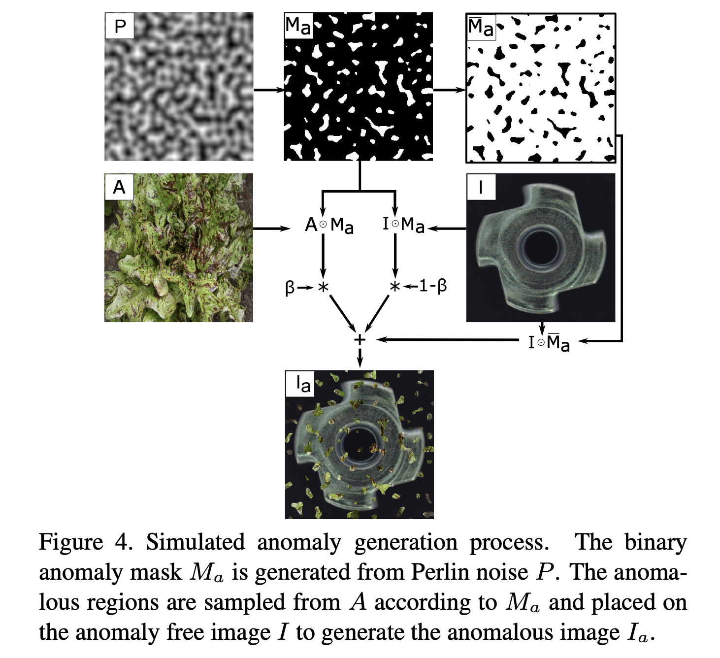
The anomaly texture source image A is sampled from an anomaly source image dataset which is unrelated to the input image distribution (Figure 4, A). Random augmentation sampling, inspired by RandAugment [10], is then applied by a set of 3 random augmentation functions sampled from the set: {posterize, sharpness, solarize, equalize, brightness change, color change, auto-contrast}.

이미지 \(A\)는 입력 이미지 분포와 무관한, 입력 이미지 분포에 포함되있지 않은 데이터셋에서 샘플링 된다. 그런 다음 \(A\)에 RandAugment에서 영감을 받은 Random augmentation sampling이 적용된다.
\(A\)에 RandAugment: {posterize, sharpness, solarize, equalize, brightness change, color change, auto-contrast} 중에서 랜덤하게 3개를 sampling하여 적용한다
posterize: 사용하는 색상의 수를 강제적으로 줄여줌으로써 이미지의 색상을 단순화시키는 동시에 이로 인해 포스터로 그린 듯한 단순한 느낌이 나도록 하는 효과
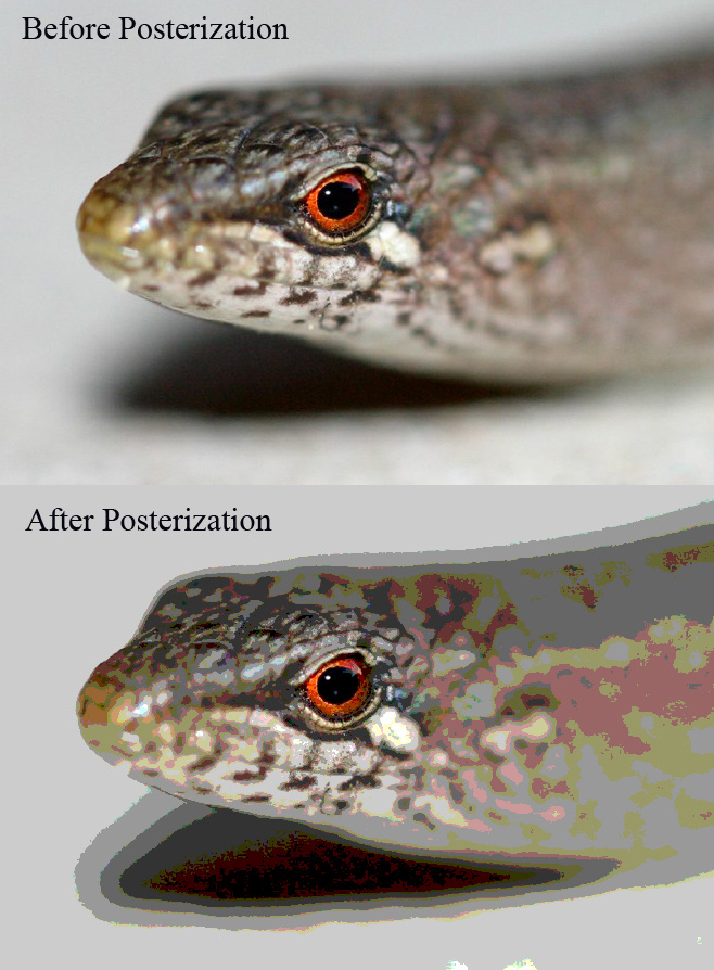
sharpness(선명도), solarize(과대 노출), equalize(평활화), brightness change(밝기 변경), color change (색상 변경), auto-contrast(명암 자동 조절)

The augmented texture image A is masked with the anomaly map Ma and blended with I to create anomalies that are just-out-of-distribution, and thus help tighten the decision boundary in the trained network. The augmented training image Ia is therefore defined as

Augmention과 anomaly map인 \(M_a\)가 적용된 이미지 \(A\)와 원본 이미지 \(I \)와 혼합되어 원본 이미지 분포에서 약간 벗어난 이상 이미지를 만들어 낸다. 따라서 훈련된 네트워크의 decision boundary을 강화하는 데 도움이 된다.(성능이 향상된다). \(M_a\)와 \(I\)와 혼합된 이미지를 \(I_a\)라고 하며 정의는 다음과 같다.

where \(\overline{M_a}\) is the inverse of \(M_a\), ⊙ is the element-wise multiplication operation and β is the opacity parameter in blending.

\(\overline{M_a}\)는 \(M_a\)의 inverse한 형태이며 ⊙는 element-wise multiplication연산이고 β는 \(I\)와 \(\overline{M_A}\)의 이미지 혼합에서 사용되는 불투명도 파라미터로 만약 A의 불투명도 파라미터 β가 0.7이라면, 최종 이미지는 A의 70%와 B의 30%를 합친 결과가 된다. 이는 A가 최종 이미지에 더 큰 영향을 미침을 의미한다.

This parameter is sampled uniformly from an interval, i.e., β ∈ [0.1, 1.0].

이 parameter는 [0.1, 1.0]에서 균일하게 랜덤으로 샘플링 된다.

The randomized blending and augmentation afford generating diverse anomalous images from as little as a single texture (see Figure 5).

랜덤으로 혼합하고 augmentation을 통해 다양한 이상 이미지를 단일 texture(\(A\))를 통해 이미지를 생성할 수 있다.

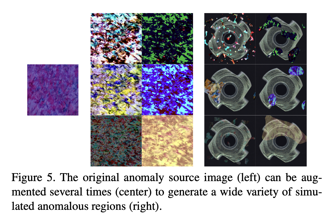
The above described simulator thus generates training sample triplets containing the original anomaly-free image \(I\), the augmented image containing simulated anomalies \(I_a\) and the pixel-perfect anomaly mask \(M_a\).

따라서 위에서 설명한 simulator는 원본 이미지(정상) \(I\), simulator 이후 비정상 이미지 \(I_a\), 이상치 마스크 \(M_a\)를 포함하는 훈련 샘플 쌍(triplets)을 생성한다.

3.4. Surface anomaly localization and detection

The output of the discriminative subnetwork is a pixel-level anomaly detection mask Mo, which can be interpreted in a straight-forward way for the image-level anomaly score estimation, i.e., whether an anomaly is present in the image.

discriminative subnetwork의 출력인 픽셀 단위의 anomaly detection mask \(M_o\)는 이미지 전체에 대한 이상 점수를 추정하는 데 사용될 수 있다.

First, \(M_o\) is smoothed by a mean filter convolution layer to aggregate the local anomaly response information.

먼저, 이상 탐지 마스크(\(M_o\))는 convolution layer에서 mean filter를 사용하여 이상치에 대한 정보를 더 극대화 시킨다. mean filter in CNN은 픽셀 값을 해당 픽셀 주변의 값들의 평균으로 대체하는 방식이다.

The final image-level anomaly score η is computed by taking the maximum value of the smoothed anomaly score map:

mean filter가 적용된 \(M_0\)에 최대값을 취하여 이상 점수 η를 계산한다. 즉, 이미지 전체에서 가장 높은 이상 점수를 가진 픽셀의 점수를 이미지 전체의 이상 점수로 사용한다는 것이다.

where \(f_{sf\times sf}\) is a mean filter of size \(sf\times sf\) and ∗ is the convolution operator.

\(f_{sf\times sf}\)는 \(sf\times sf\) 크기의 mean filter라는 것을 의미하고 *은 CNN 연산자를 의미한다.

In a preliminary study, we trained a classification network for the image-level anomaly classification, but did not observe improvements over the direct score estimation method (5).

이전 연구에서, Image-level anomaly classification에서의 결과는 direct score estimation method는 개선된 결과를 보지 못했다
이미지 수준의 이상 분류(Image-level anomaly classification): 전체 이미지를 기반으로 이상을 분류하는 방법으로 예를 들어, 공장에서 생산되는 제품의 이미지를 분석하여 제품에 결함이 있는지 없는지를 판단하는 것이 이에 해당된다.
직접적인 점수 추정 방법(Direct score estimation method): 이상 점수 맵에서 최대 이상 점수를 추출하여 이미지 전체의 이상 점수를 계산하는 방법으로 이 방법은 각 픽셀에 대한 이상 점수를 계산한 후, 이 점수들을 종합하여 이미지 전체의 이상 점수를 추정한다. 이 방법은 픽셀 수준에서 이상을 탐지하므로, 이상이 발생한 구체적인 위치를 파악하는 데 유용하다.

Experiments

Image-level AUROC is used for anomaly de- tection and a pixel-based AUROC for evaluating anomaly localization.

We thus additionally report the pixel-wise average precision metric (AP), which is more appropriate for highly imbalanced classes and in particular for surface anomaly detection, where the precision plays an important role.

Datasets

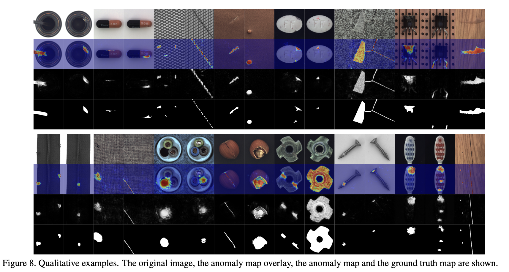
MVTec(15 classes)

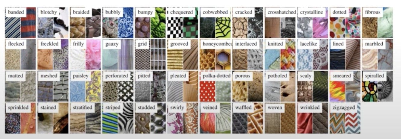
DTD(Describable Textures Dataset)

Use Anomaly source dataset. Consisting of 5640 images, organized according to a list of 47 terms (categories).

Setting

The network is trained for 700 epochs on the MVTec anomaly detection dataset.

The learning rate is set to \(10^{-4}\) and is multiplied by 0.1 after 400 and 600 epochs.

Image rotation in the range of (−45, 45) degrees is used as a data augmentation method on anomaly free images during training to alleviate overfitting due to the relatively small anomaly-free training set size.

Surface Anomaly Detection

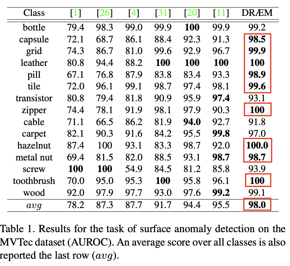
AUROC를 지표로 하여 나타난 결과로 MVTec dataset에서 15개의 class중 9개의 class에 대해서 가장 높은 성능을 달성 했다. [1] GANomaly, [26] DAGAN, [4] Student-Teacher AD, [31] RIAD, [20] Gaussian AD, [11] Padim 순으로 비교하면 된다.

Anomaly localization

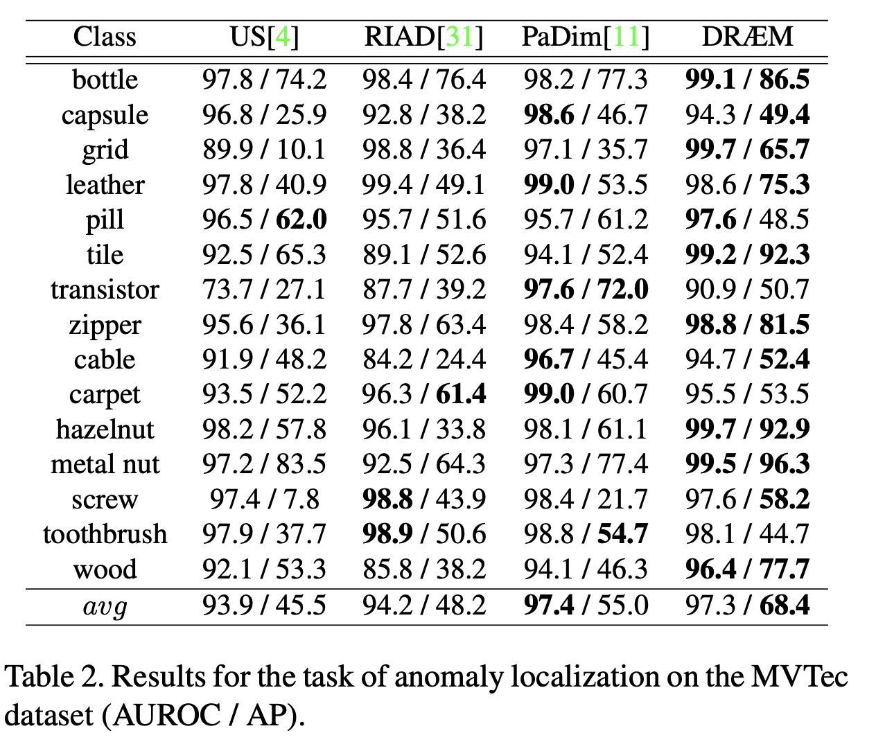
Anomaly localization에서의 MVTec dataset의 결과로 평가 지표는 (AUROC/ AP) 이다.

15개의 class중 11개의 class에서 가장 높은 AP(Average Precision)스코어를 얻었다.

Ablation Study

Architecture

Disc. 를 보면 Reconstruction Subnetwork를 제거한 후 Discriminative subnetwork만을 학습시켜 평가한다. 성능 하락이 보이는데 그 이유는 simulated anomalies에 discriminative subnetwork가 overfitting되기 때문이다.
Recon. -AE에서는 reconstructive subnetwork만을 남기고 discriminative subnetwork 제거하여 성능을 평가하고 있다..
Recon-AE(MSGMS)에서는 유사도 함수를 SSIM이 아닌 MS-GMS로 사용하였을 때의 성능지표이다. 그러나 기존 SSIM을 Draem에 적용한 것이 더 높은 성능을 보였다.
Bozicet al. 에서는 DRÆM의 backbone을 최신 SOTA supervised surface anomaly detection network로 대체하고, 평가했으나 성능이 크게 떨어졌다. 그 이유는 정상이나 이상치의 모습 자체를 학습하는 것보다 기존 Draem에서 소개되었던 정상이미지와 비정상이미지가 얼마나 벗어났는지를 학습하는 것이 더 효과적이다라는 것을 보여준다.
DRAEM_no_aug, DRAEM_aug에서는 크게 차이가 나지 않으나 β(the opacity parameter)를 적용한 것과는 꽤나 차이가 있음을 볼 수 있다.

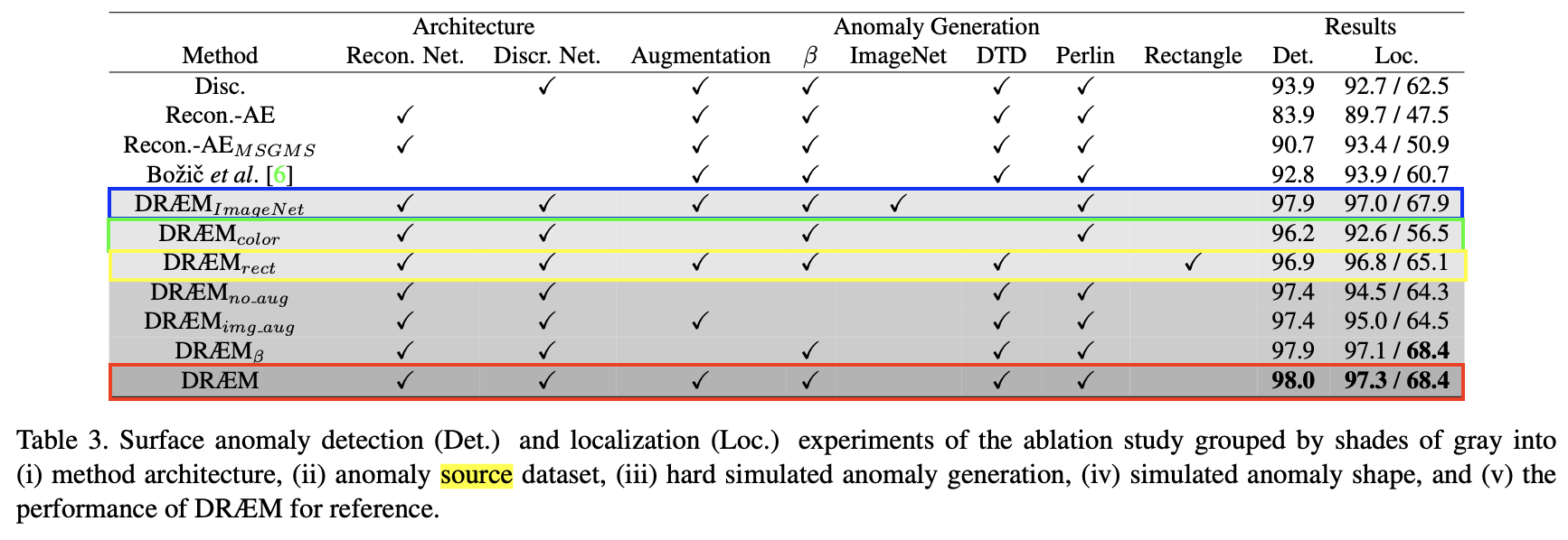
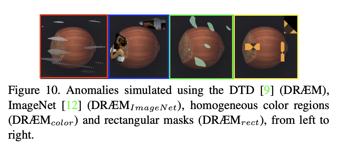
아래 색깔친 박스는 Texture source image from an anomaly source image dataset에 따른 실험한 결과를 보여준다.

아래 그림에서 빨강박스는 DRAEM에 Texture source dataset으로 DTD dataset을 적용한 결과
파란색 박스는 DRAEM에 Texture source dataset으로 ImageNet을 적용한 결과
초록색 박스는 DRAEM에 random하게 sampling된 색으로 적용한 결과
노란색 박스는 DRAEM에 random하게 sampling된 직사각형을 적용한 결과이고 이 결과가 Navie DRAEM과 비교해 볼 때 약간의 성능차이만 있었기 때문에 Simulated로 부터 나온 Anomaly의 모양이 실제 Anomaly모양과 비슷하지 않아도 된다는 것이다.

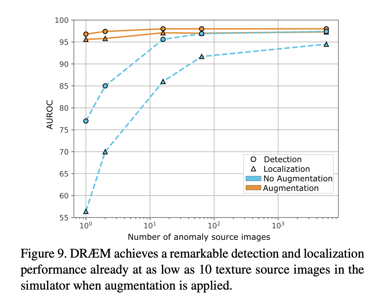
Anomaly source dataset으로 이용되는 데이터 크기에 따른 성능을 평가한 결과이다.

위 결과에서 볼 수 있듯이 β(the opacity parameter)와 Augmentation의 성능에 크게 영향을 주고 있으며 적은 수의 Texture source image로도 높은 성능을 달성할 수 있다고 말한다.

Comparison with supervised methods

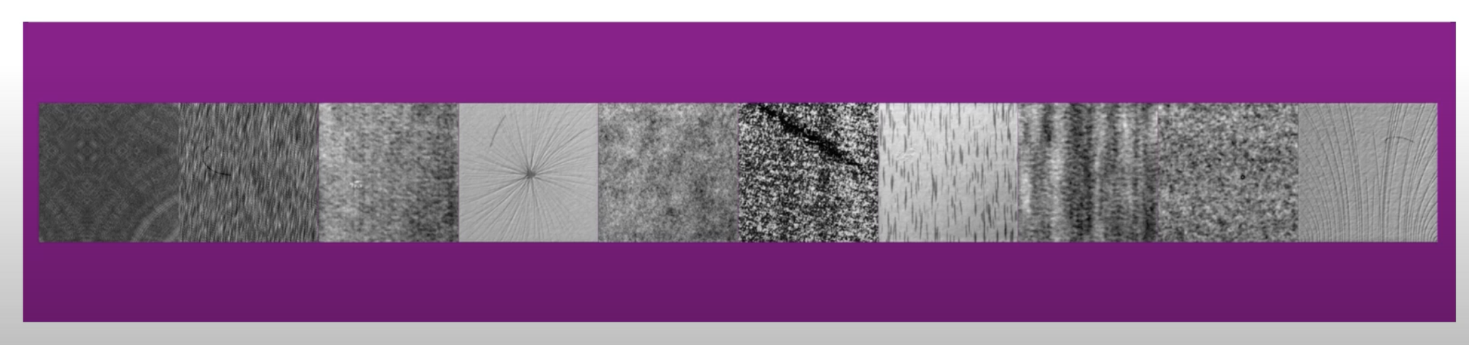
We thus compare DRÆM with the supervised methods on the DAGM dataset [28] that contains 10 textured object classes.

DAGM dataset

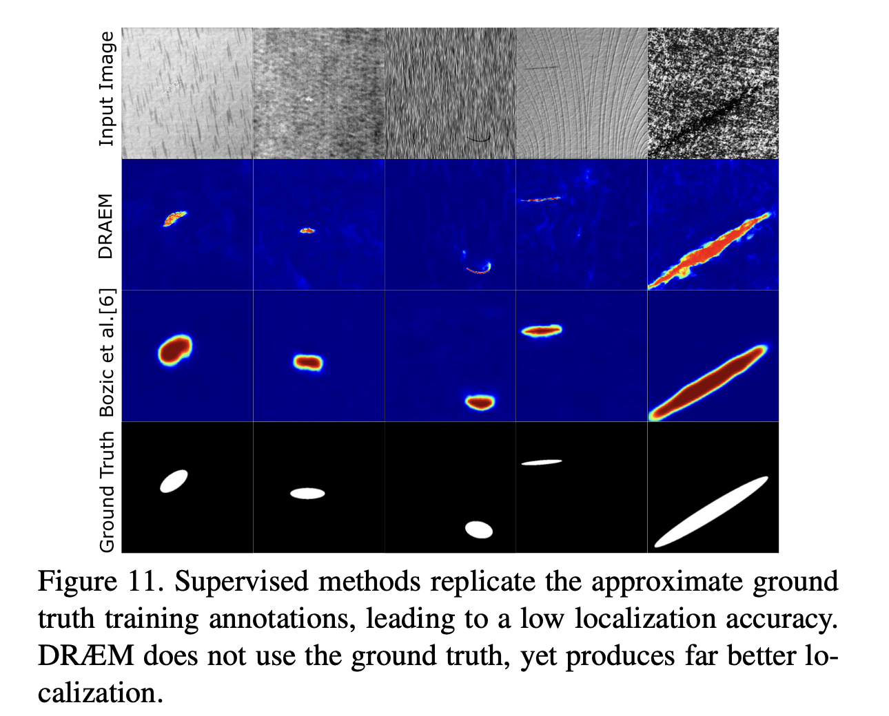
Supervised Learning에서의 Draem은 surface anomaly을 대략적으로 타원의 형태로 cover하고 있는 모습을 볼 수 있다.(Bozic et al.)

그 이유는 대략적으로 라벨링(coarsely annotated) 되었기 때문에, 테스트 이미지에서도 anomaly한 부분을 정확하게 segmentation하기는 어렵다. 아래 보면 Ground Truth를 정답으로 학습하여 테스트한 Bozic et al.행의 결과와 unsupervised로 학습된 DRAEM의 결과 차이를 보면 알 수 있다.

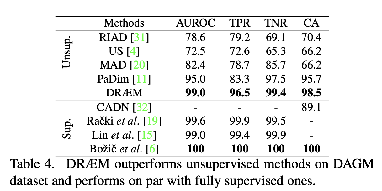
또한 Unsupervised Learning이 Supervised Learning과 거의 준하는 결과를 보여준다.

DRÆM – A discriminatively trained reconstruction embedding for surface anomaly detection 논문 전체 번역

서론

목차