DenseNet 논문리뷰

서론

• Gao Huang, Zhuang Liu, Laurens van der Maaten, Kilian Q. Weinberger; Proceedings of the IEEE Conference on Computer Vision and Pattern Recognition (CVPR), 2017, pp. 4700-4708 Densely Connected Convolutional Networks
• 논문에서 제안하는 Dense connection(concatenating)을 중심으로 살펴본다.

목차

1. Abstract
2. Introduction
   1. background Research
   2. Recent Research
   3. Propose
   4. Related Paper
3. Related Work
4. DenseNet
   1. ResNets.
   2. Dense connectivity.
   3. Composite function.
   4. Pooling layers.
   5. Growth rate.
   6. Bottleneck layers.
   7. Compression.
   8. Implementatoin Details.
5. Experiments
   1. Datasets
      1. CIFAR.
      2. SVHN.
      3. ImageNet.
   2. Training
   3. Classification Results on CIFAR and SVHN
      1. Accuracy.
      2. Capacity
      3. Parameter Efficiency.
      4. Overfitting.
   4. Classification Results on ImageNet
6. Discussion
   1. Model compactness.
   2. Implicit Deep Supervision.
   3. Stochastic vs. deterministic connection.
   4. Feature Reuse.
7. Conclusion

Abstract

• Recent work has shown that convolutional networks can be substantially deeper, more accurate, and efficient to train if they contain shorter connections between layers close to the input and those close to the output.
• 최근 연구에 따르면 Input, output layer에 short connection을 Convolution Networks에 사용하면 상당히 깊고, 정확하며 훈련하기 효율적이다.
• In this paper, we embrace this observation and introduce the Dense Convolutional Network (DenseNet), which connects each layer to every other layer in a feed-forward fashion.
• 본 논문에서는 최근 연구에 따라 feedforward 방식에서 각 layer들이 모든 다른 layer와 connection를 두는 DenseNet을 소개한다.
• Whereas traditional convolutional networks with L layers have L connections—one between each layer and its subsequent layer-our network has L(L+1)2 direct connections.
• 이제까지는 layer가 그 다음 하위 레이어와의 연결 구조를 갖는 CNN과는 달리 DenseNet은 \(\frac{L(L+1)}{2}\) 의 direct connection을 갖는 새로운 구조다.
• For each layer, the feature-maps of all preceding layers are used as inputs, and its own feature-maps are used as inputs into all subsequent layers.
• 앞 layer에서 얻은 모든 feature map은 계속해서 뒤 layer의 입력으로 입력되는 구조다.
• DenseNets have several compelling advantages: they alleviate the vanishing-gradient problem, strengthen feature propagation, encourage feature reuse, and substantially reduce the number of parameters.
• DenseNet은 몇 가지 강력한 이점이 있다.
  1. vanishing gradient를 방지
  2. feature propagation을 강화.
  3. feature의 재사용성.
  4. 파라미터 수 감소.
• We evaluate our proposed architecture on four highly competitive object recognition benchmark tasks (CIFAR-10, CIFAR-100, SVHN, and ImageNet). DenseNets obtain significant improvements over the state-of-the-art on most of them, whilst requiring less computation to achieve high performance.
• 4개의 대표적인 Dataset(cifar-10, cifar-100, SVHN, ImageNet)에서 모두 좋은 성능을 거두었으며, 당시 state-of-the-art의 성능이면서도 엄청난 계산 복잡도를 낮추었다.

Introduction

background Research

• As CNNs become increasingly deep, a new research problem emerges: as information about the input or gradient passes through many layers, it can vanish and “wash out” by the time it reaches the end (or beginning) of the network.
• CNN이 점점 더 깊어짐에 따라 Input 또는 gradient가 layer를 거칠수록 정보를 잃어버리는 문제가 발생한다.

Recent Research

• Many recent publications address this or related problems. ResNets and Highway Networks bypass signal from one layer to the next via identity connections.
• 이러한 문제를 해결하기 위해 ResNet과 Highway Networks는 Residual connecntion을 사용한다.
• Stochastic depth shortens ResNets by randomly dropping layers during training to allow better information and gradient flow.
• Stochastic depth를 ResNet의 깊이를 줄이는 방식으로 layer를 무작위로 생략함으로써 Input 정보와 gradient 흐름을 개선한다.
• FractalNets repeatedly combine several parallel layer sequences with different number of convolutional blocks to obtain a large nominal depth, while maintaining many short paths in the network. Although these different approaches vary in network topology and training procedure, they all share a key characteristic: they create short paths from early layers to later layers.
• FractalNets은 Network의 깊이를 늘리기 위해 여러 short connection을 추가하며 layer들이 병렬로 구성된 convolution block을 사용한다. 이러한 접근 방식은 앞 단의 layer정보를 잘 보존할 수 있다.

Propose

• In this paper, we propose an architecture that distills this insight into a simple connectivity pattern: to ensure maximum information flow between layers in the network, we connect all layers (with matching feature-map sizes) directly with each other.
• 이 논문에서는, 네트워크 내의 layer들에 대한 정보를 최대한 보존하기 위해, 모든 layer들을 서로 간단하게 연결 시키는 구조를 갖는 아키텍처를 제안한다.

Related Paper

• Kaiming He, et al., "Deep Residual Learning for Image Recognition"

Related Work

• DenseNet과 비슷한 구조를 갖는 Highway Network, GoogleNet, ResNet, FractalNet 등이 네트워크 구조가 갖는 특징을 가지고 성능을 향상시켰는지에 대해서 설명한다.
• 위 부분은 생략하고 넘어가며 아래는 DeseNet위주로 정리하였다.
• Instead of drawing representational power from extremely deep or wide architectures, DenseNets exploit the potential of the network through feature reuse, yielding condensed models that are easy to train and highly parameter efficient.
• DenseNets는 앞에서 설명한 깊거나 넓은 구조를 이용해 성능을 높이는 모델들과는 달리 feature 재사용을 통해 parameter의 효율성을 높이고 훈련하기 쉬운 모델을 생성한다.
• Concatenating feature-maps learned by different layers increases variation in the input of subsequent layers and improves efficiency.
• 서로 다른 layer들에 의해 학습된 feature map들을 concat함으로써, layer들의 Input에 변화가 증가하고, 효율성 또한 향상된다.
• This constitutes a major difference between DenseNets and ResNets. Compared to Inception networks, which also concatenate features from different layers, DenseNets are simpler and more efficient.
• ResNet뿐만 아니라, 다른 Layer들을 concatenate하는 Inception Network의 경우와 비교했을 때에도 DenseNet은 더 단순하고 효율적인 구조를 갖는다.

DenseNet

• Consider a single image \(x_0\) that is passed through a convolutional network.
• 단일 이미지 \(x_0\)가 convolution network를 통과한다고 하자
• The network comprises L layers, each of which implements a non-linear transformation \(H_l(\cdot)\), where indexes the layer.
• Network는 L개의 layer로 구성되어있고 각 Layer에서는 non-linear transformation인 \(H_l(\cdot)\)를 수행한다(\(l\)은 layer의 index를 의미)
• \(H_l(\cdot)\) can be a composite function of operations such as Batch Normalization (BN), rectified linear units (ReLU), Pooling, or Convolution (Conv).
• \(H_l(\cdot)\)은 BN, ReLU, Pooling, Convolution 등과 같은 함수로 이뤄져있다.
• We denote the output of the \(l^{th}\) layer as \(x_l\).
• \(l\)번째 Layer의 결과를 \(x_l\) 이라 하자.

ResNets.

• Traditional convolutional feed-forward networks connect the output of the \(l^{th}\)layer as input to the\((l+1)^{th}\), which gives rise to the following layer transition: \(x_l =H_l(x_{l-1}).\)
• 기존의 Convolutional feed-forward network는 \(l\)번째 Layer의 output을 그 다음 Layer인 \((l+1)\)번째 Layer의 Input으로 연결한다. 식으로 나타내면 다음과 같다: \(x_l =H_l(x_{l-1}).\)
• ResNets add a skip-connection that bypasses the non-linear transformations with an identity function:
• ResNet은 identity function을 통해 non-linear transformation을 건너뛰는 skip connection을 추가한다 :

• An advantage of ResNets is that the gradient can flow directly through the identity function from later layers to the earlier layers.
• ResNet의 장점은 identity function을 통해 이후의 Layer에서 이전의 Layer로 gradient가 직접적으로 흐를 수 있다는 점이다.
• However, the identity function and the output of \(H_l\) are combined by summation, which may impede the information flow in the network.
• 하지만 identity function과 \(H_l\)의 output이 summation을 통해 결합되면서 네트워크의 information flow를 방해할 수도 있다.

Dense connectivity.

• To further improve the information flow between layers we propose a different connectivity pattern: we introduce direct connections from any layer to all subsequent layers.
• Layer들 간의 information flow를 향상시키기 위해, 본 논문에서는 다른 connectivity pattern을 제안했다: 모든 Layer를 연결하는 방식이다.
• Figure 1 illustrates the layout of the resulting DenseNet schematically.
• Figure 1은 Densenet의 구조를 보여준다.

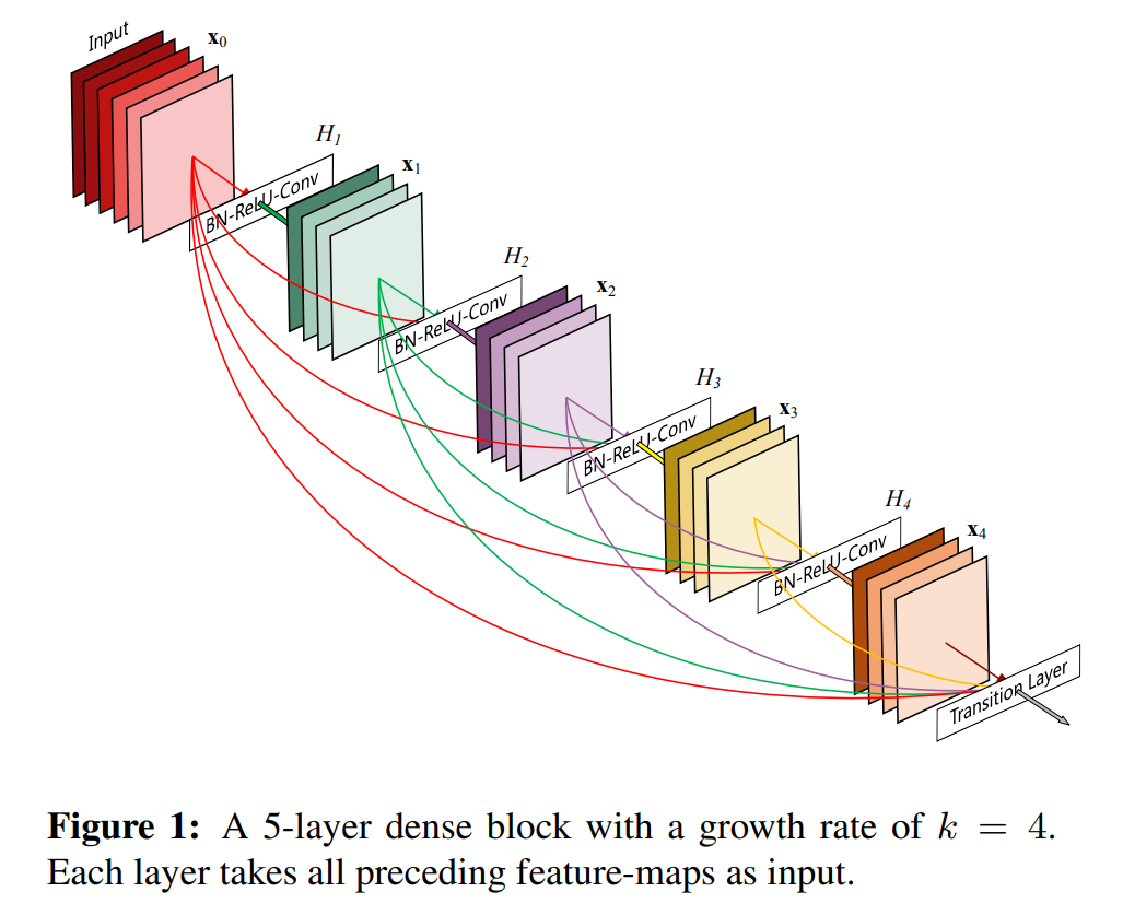
• Consequently, the \(l^{th}\) layer receives the feature-maps of all preceding layers, \(x_0, ..., x_{l-1}\) as input:
• 결과적으로, \(l\)번째 Layer는 이전의 모든 Layer들의 feature map(\(x_0, ..., x_{l-1}\))을 input으로 받게 된다 :

• where \([x_0, x_1, ... , x_{l-1}]\) refers to the concatenation of the feature-maps produced in layers 0, \(0, ...\;,l-1\).
• 위 식에서 \([x_0, x_1, ... , x_{l-1}]\)은 각 Layer에서 만들어진 feature map들의 concatenation이다.
• Because of its dense connectivity we refer to this network architecture as Dense Convolutional Network (DenseNet).
• 이러한 dense connectivity 때문에, 이러한 구조를 DenseNet이라 명명했다.
• For ease of implementation, we concatenate the multiple inputs of \(H_l(\cdot)\) in eq. (2) into a single tensor.
• 구현의 용의성을 위해, 여러 inputs을 \(H_l(\cdot)\) 통해 단일 tensor로 concatenate 한다.

Composite function.

• Motivated by [12], we define \(H_l(\cdot)\) as a composite function of three consecutive operations: batch normalization (BN) [14], followed by a rectified linear unit (ReLU) [6] and a 3 × 3 convolution (Conv).
• 다른 연구에서 영감을 받아, \(H_l(\cdot)\)을 다음 3가지 operation의 합성함수로 정의했다: BN, ReLU, 3 x 3Convolution.

Pooling layers.

• The concatenation operation used in Eq. (2) is not viable when the size of feature-maps changes.
• 위의 식(2)에서 사용된 concatenation 연산은 feature map의 사이즈가 바뀌면 사용할 수 없다.
• However, an essential part of convolutional networks is down-sampling layers that change the size of feature-maps.
• 하지만, Convolutional network의 down-sampling Layer를 통해 feature map의 사이즈를 바꿀 수 있다.
• To facilitate down-sampling in our architecture we divide the network into multiple densely connected dense blocks; see Figure 2.
• down-sampling을 용이하게 하기 위해, 네트워크를 서로 밀집하게 연결된 여러개의 dense block으로 나누었다. Figure 2를 봐보자.
• We refer to layers between blocks as transition layers, which do convolution and pooling.
• 각 Block 사이에서 Convolution과 Pooling을 수행하는 Layer를 Transition Layer라고 한다.

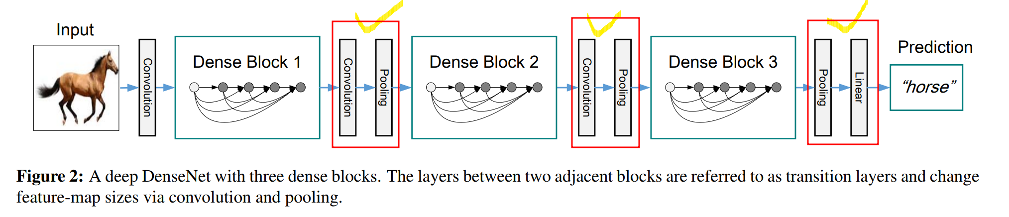
• The transition layers used in our experiments consist of a batch normalization layer and an 1×1 convolutional layer followed by a 2×2 average pooling layer.
• Transition Layer는 Batch Normalization Layer, 1 x 1 Convolutional Layer, 그리고 2 x 2 Pooling Layer로 구성되어있다.

Growth rate.

• If each function \(H_l\) produces \(k\) featuremaps, it follows that the \(l^{th}\) layer has \(k_0 + k\times(l-1)\) input feature-maps, where \(k_0\) is the number of channels in the input layer.
• 만약 각각의 함수 \(H_l\)이 \(k\)개의 feature map을 만든다고 하면, \(l\)번째 Layer의 feature map의 개수는 \(k_0 + k\times(l-1)\) 개가 될 것이다. (\(k_0\)는 Input layer의 채널 수)
  • Input layer인 \(H_1\)에서 \(k_0\)개의 feature map이 생긴다
  • \(H_1\)에서 \(k_0\)개와 \(H_2\)에서 \(k\)개의 feature map이 생김으로 총 \(k_0+k\)개가 된다.
  • \(H_3\)에서는 \(k\)개와 \(H_1\)와 \(H_2\)에서 만들어진 \(k_0+k\)개의 feature map이 생김으로 총 \(k_0+2k\)개가 된다.
  • 즉, \(H_l\) 에서는 \(k_0+(l-1)k\)개 feature map을 생성한다.
• An important difference between DenseNet and existing network architectures is that DenseNet can have very narrow layers, \(e.g., k=12.\)
• DenseNet과 기존 네트워크 구조들 간의 차이점은, DenseNet이 비교적 좁은 Layer를 가졌다는 것이다. \((k=12)\)
• We refer to the hyperparameter k as the growth rate of the network.
• 여기서 이 \(k\)를 네트워크의 Growth Rate라고 한다.
  • Growth Rate: 각 Layer에서 몇 개의 feature map을 생성하는 피처 맵의 수를 의미
• We show in Section 4 that a relatively small growth rate is sufficient to obtain state-of-the-art results on the datasets that we tested on.
• 비교적 작은 growth rate로 아래 table2는 각 dataset에 대해 SOTA를 달성하기에 충분하다는 것을 보여준다.

• One explanation for this is that each layer has access to all the preceding feature-maps in its block and, therefore, to the network’s “collective knowledge”.
• SOTA인 이유에 대해서 설명하면 각 layer들이 이전 block들에 대해 feature-maps에 접근이 가능함으로 이를 네트워크의 “collective knowledge”라고 한다.
• One can view the feature-maps as the global state of the network.
• feature-map을 통해 network가 어떻게 학습되고 있는지를 볼 수 있다.
• Each layer adds k feature-maps of its own to this state.
• 각 layer들은 k개의 feature-map들을 현재 state에 추가한다.
• 각 레이어가 k(growth rate)만큼의 자체 피처 맵을 현재 상태(이전 레이어들의 출력)에 추가한다는 의미다
• 쉽게 말하면 각 레이어가 출력하는 피처 맵이 이전 레이어의 출력과 결합(concatenated)되어 다음 레이어의 입력으로 사용된다는 것을 나타낸다.
• The growth rate regulates how much new information each layer contributes to the global state.
• global state(모든 층에서 공유되는 정보 상태=feature map)에 기여하는 새로운 정보의 양(feature map)은 growth rate가 조절한다.
• The global state, once written, can be accessed from everywhere within the network and, unlike in traditional network architectures, there is no need to replicate it from layer to layer.
• 한번 global state에 입력된 정보는 네트워크의 어디에서나 접근이 가능하며, 전통적인 네트워크 구조와 달리 각 층에서 그 정보를 복제할 필요가 없다.

Bottleneck layers.

• Although each layer only produces \(k\) output feature-maps, it typically has many more inputs.
• 각 Layer들은 k개의 output feature map을 생성하지만, 일반적으로 그에 비해 더 많은 input이 필요하다.
• It has been noted in ResNet, Inception Net that a 1×1 convolution can be introduced as bottleneck layer before each 3×3 convolution to reduce the number of input feature-maps, and thus to improve computational efficiency.
• ResNet, Incepction Net에서 언급했듯이 bottleneck 구조는 1x1convoltion을 통해 3x3convolution에서의 input을 줄임으로서 computational efficiency를 높일 수 있다.
• We find this design especially effective for DenseNet and we refer to our network with such a bottleneck layer, i.e., to the BN-ReLU-Conv(1×1)-BN-ReLU-Conv(3×3) version of \(H_l\), as DenseNet-B.
• 우리는 이러한 설계가 DesNet에서도 효과적인 것을 발견했고 DenseNet에 이러한 Bottleneck 구조를 사용했다.
• In our experiments, we let each 1×1 convolution produce 4\(k\) feature-maps.
• 실험에서 우리는 각 1x1convolution에서 4k의 featuremap을 생성한다.

Compression.

• To further improve model compactness, we can reduce the number of feature-maps at transition layers.
• 모델의 compactness(간결함?)을 향상시키기 위해, transition Layer에서 feature map의 개수를 줄일 수 있다.
• If a dense block contains \(m\) feature-maps, we let the following transition layer generate \([\theta m]\) output featuremaps, where \(0<\theta \leq 1\) is referred to as the compression factor.
• 만약 dense block이 m개의 feature map을 가지고 있다면, 그 뒤의 transition Layer는 θm개의 output feature map을 반환할 것이다. 여기서, θ가 바로 compression factor이다. (단, 0 < θ <= 1)
• We refer the DenseNet with \(\theta <1\) as DenseNet-C, and we set \(\theta = 0.5\) in our experiment.
• 만약 θ < 1 인 경우, 이러한 DenseNet은 DenseNet-C라고 하며, 본 논문에서는 θ = 0.5 로 설정했다.
• When both the bottleneck and transition layers with \(\theta <1\) are used, we refer to our model as DenseNet-BC.
• bottleneck, transition Layer 모두 θ < 1 인 경우, DenseNet-BC라고 명명했다.

Implementatoin Details.

• On all datasets except ImageNet, the DenseNet used in our experiments has three dense blocks that each has an equal number of layers.
• ImageNet dataset을 제외한 dataset으로 학습된 DenseNet은 모두 동일한 개수의 Layer를 가진 3개의 Dense Block으로 구성된다.
• Before entering the first dense block, a convolution with 16 (or twice the growth rate for DenseNet-BC) output channels is performed on the input images.
• 첫 번째 Dense Block을 들어가기 전, input image에 대해 convolution으로 16개의 output channel을 갖도록 수행했다.(또는 DenseNet-BC의 경우 growth rate를 2배로 한다)
• For convolutional layers with kernel size 3×3, each side of the inputs is zero-padded by one pixel to keep the feature-map size fixed.
• feature map size를 유지하기 위해서, kernel_size가 3x3인 convolution에서의 input에 zero-padding을 1로 설정 했다.
• We use 1×1convolution followed by 2×2 average pooling as transition layers between two contiguous dense blocks.
• 인접한 두 Dense Block 사이의 Transition Layer로는 1x1 Convolution, 2x2 average pooling을 사용했다.
• At the end of the last dense block, a global average pooling is performed and then a softmax classifier is attached.
• 마지막 Dense Block의 끝에는 global average pooling, softmax classifier가 실행된다.
• The feature-map sizes in the three dense blocks are 32x32, 16x6, and 8x8, respectively.
• 3개의 Dense Block의 feature map size는 각각 32x32, 16x16, 8x8이다.
• We experiment with the basic DenseNet structure with configurations {L = 40, k = 12}, {L =100, k = 12} and {L = 100, k = 24}.
• DenseNet 구조의 총 층 수가 40, 100, 100이고 growth rate가 각각 12, 12, 24인 세 가지 설정으로 실험했다.
• For DenseNetBC, the networks with configurations {L = 100, k = 12}, {L= 250, k= 24} and {L= 190, k= 40} are evaluated.
• DenseNetBC 구조의 총 층 수가 100, 250, 190이고 growth rate가 각각 12, 24, 40인 세 가지 설정으로 평가했다.
• In our experiments on ImageNet, we use a DenseNet-BC structure with 4 dense blocks on 224×224 input images.
• ImageNet dataset에 대한 DenseNet은 DenseNet-BC를 사용했고 224x224 image를 input으로 하며, Dense Block의 개수는 4개이다.
• The initial convolution layer comprises convolutions of size 7×7 with stride 2; the number of feature-maps in all other layers also follow from setting k.
• 초기 convolution layer는 2k개의 featuremap과 7x7의 kernel_size를 갖고 stride=2로 설정한다 그리고 다른 모든 layer의 feature map또한 k로 설정한다.
• The exact network configurations we used on ImageNet are shown in Table 1.
• 자세한 네트워크 구성은 아래 Table1을 참고한다.

Experiments

• We empirically demonstrate DenseNet’s effectiveness on several benchmark datasets and compare with state-of-theart architectures, especially with ResNet and its variants.
• DenseNet의 효과를 입증하기 위해 여러 데이터셋에 대해 실험을 진행했으며, ResNet과 같은 최신 성능을 갖는 모델과 비교했다.

Datasets

CIFAR.

The two CIFAR datasets consist of colored natural images with 32×32 pixels.

• 두 개의 CIFAR dataset(32 x 32 pixel의 color 이미지)을 사용했다.

CIFAR-10 (C10) consists of images drawn from 10 and CIFAR-100 (C100) from 100 classes.

• CIFAR-10(C10)은 10개의 class로 구성되어 있으며 CIFAR-100(C100)은 100개로 구성되어있다.

The training and test sets contain 50,000 and 10,000 images respectively, and we hold out 5,000 training images as a validation set.

• training, test set은 각각 50,000, 10,000개이며, training set 중 5,000개는 validation에 사용했다.

We adopt a standard data augmentation scheme (mirroring/shifting) that is widely used for these two datasets.

• 두 Dataset에서 Data augmentation방식으로는 가장 표준적인 mirroring/shifting 을 사용했다.

We denote this data augmentation scheme by a “+” mark at the end of the dataset name (e.g., C10+).

• data augmentation을 거친 dataset의 이름에는 "+" 기호를 붙였다.(ex) C10+)

For preprocessing, we normalize the data using the channel means and standard deviations.

• 전처리로는 channel의 평균과 표준편차를 이용하여 데이터를 정규화했으며,

For the final run we use all 50,000 training images and report the final test error at the end of training.

• 최종 실행 시 50,000개의 data를 모두 사용하고 training이 끝나면 최종 test error를 report 했다.

SVHN.

The Street View House Numbers (SVHN) dataset [24] contains 32×32 colored digit images.

• Street View House Numbers (SVHN) dataset(32 x 32 pixel의 color 이미지)을 사용했다.

There are 73,257 images in the training set, 26,032 images in the test set, and 531,131 images for additional training.

• training은 73,257, test set는 26,032개이며, 추가적인 training을 위해 531,131개의 이미지를 사용했다.

Following common practice we use all the training data without any data augmentation, and a validation set with 6,000 images is split from the training set.

• Data augmentation없이 training을 진행했으며, training set 중 6,000개는 validation에 이용했다.

We select the model with the lowest validation error during training and report the test error.

• training 중 가장 낮은 validation error를 보인 모델을 선택하고 test error를 report 했다.

We follow [42] and divide the pixel values by 255 so they are in the [0, 1] range.

• 추가적으로, 픽셀값이 [0, 1] 범위 내에 있도록 255로 나눠주었다.

ImageNet.

The ILSVRC 2012 classification dataset consists 1.2 million images for training, and 50,000 for validation, from 1,000 classes.

• ILSVRC 2012 classification dataset을 사용했으며, training은 1.2million validation set은 50,000개이며, 1,000개의 class로 나뉜다.

We adopt the same data augmentation scheme for training images as in [8, 11, 12], and apply a single-crop or 10-crop with size 224×224 at test time.

• 모든 training image에 대해 동일한 data augmentation을 적용했으며, test시 single-crop 또는 10-crop(with size 224 x 224) 를 적용했다.

Following [11, 12, 13], we report classification errors on the validation set.

• classification error는 validation set의 결과를 바탕으로 했다.

Training

Optimization : SGD

Batch size : 64(CIFAR & SVHN), 256(ImageNet)

Epoch : 300(CIFAR), 40(SVHN), 90(ImageNet)

Learning rate : 0.1

(CIFAR & SVHN : divided by 10 at 50% and 75% of the total number of training epochs)

(ImageNet : lowered by 10 times at epoch 30 and 60)

Wight Decay : 0.0001 (Nesterov Momentum of 0.9)

Dropout : 0.2 (C10, C100, SVHN)

Classification Results on CIFAR and SVHN

We train DenseNets with different depths, L, and growth rates, k.

• 서로 다른 깊이(L)및 growth rate(k)로 DenseNet 훈련을 진행했다.

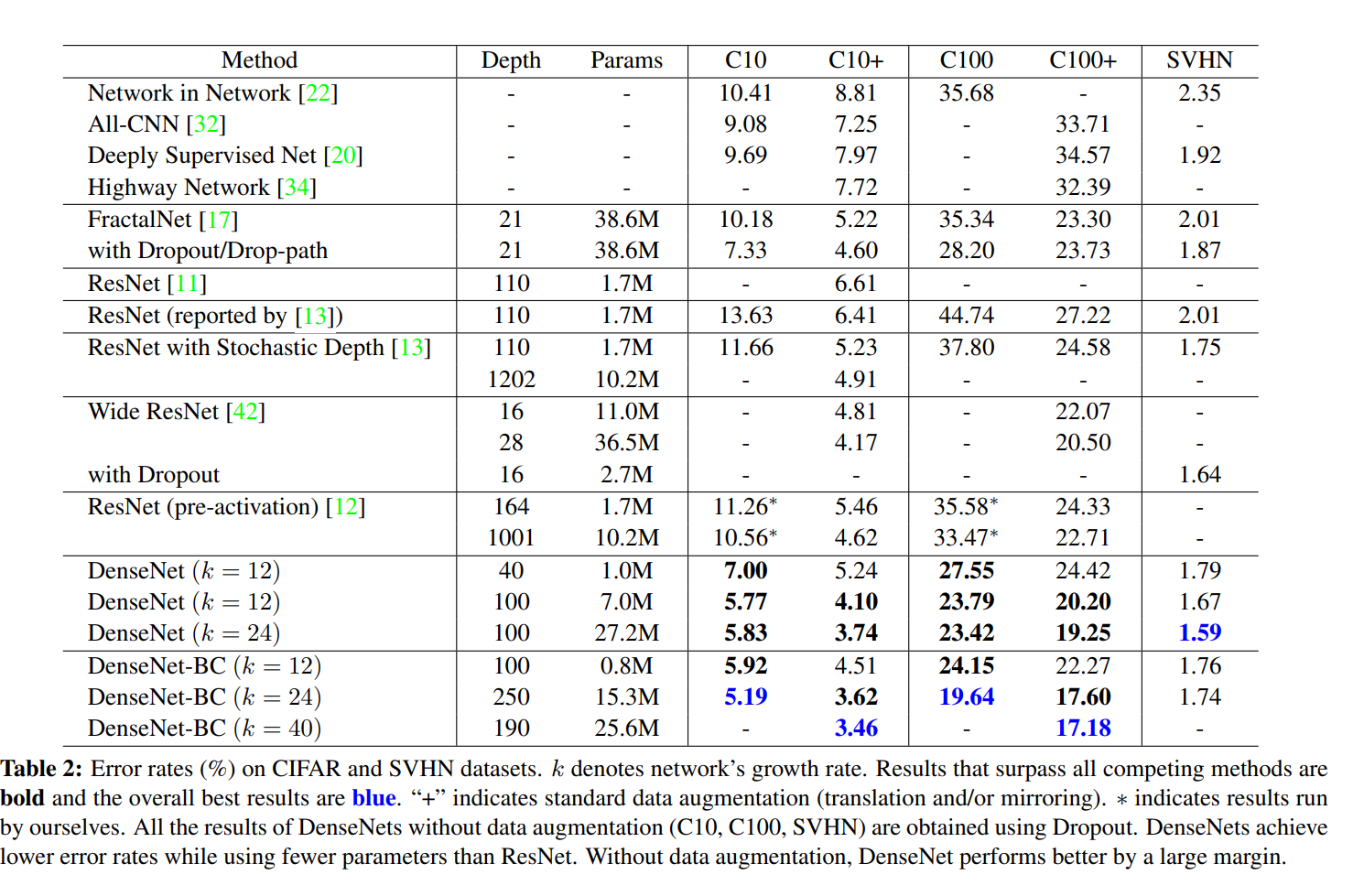
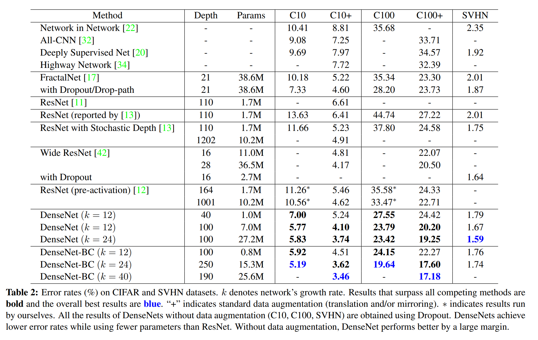
The main results on CIFAR and SVHN are shown in Table 2.

• CIFAR, SVHN에 대한 결과는 Table2. 를 참고하자.

To highlight general trends, we mark all results that outperform the existing state-of-the-art in boldface and the overall best result in blue.

• general trends를 나타내기 위해 기존 기술보다 높은 성능을 보인 결과는 굵은 글씨로 표기하였으며, 전체적으로 최상의 결과를 보인 네트워크는 파란색으로 표기했다.

Accuracy.

Possibly the most noticeable trend may originate from the bottom row of Table 2, which shows that DenseNet-BC with L = 190 and k = 40 outperforms the existing state-of-the-art consistently on all the CIFAR datasets.

• 가장 주목할만한 trend는 Table 2.의 가장 아래줄에서 확인할 수 있다, DenseNet-BC, 그 중에서도 특히 Layer가 190개, k(growth rate)가 40개의 경우 CIFAR dataset에 대해 기존보다 훨씬 높은 성능을 보였다.

Its error rates of 3.46% on C10+ and 17.18% on C100+ are significantly lower than the error rates achieved by wide ResNet architecture [42].

• C10+, C100+에서 각각 3.46, 17.18%의 error rate를 보였으며, 이는 wide ResNet 구조에서 달성한 error rate보다 훨씬 낮은 수치이다.

Our best results on C10 and C100 (without data augmentation) are even more encouraging: both are close to 30% lower than FractalNet with drop-path regularization [17].

• C10과 C100(without data augmentation)에 대한 결과는 더욱 놀랍다. 두 경우에 대한 결과 모두 drop-path regularization을 사용한 Fractal Net보다 30% 가까이 낮았다.

On SVHN, with dropout, the DenseNet with L = 100 and k = 24 also surpasses the current best result achieved by wide ResNet.

• dropout을 사용한 SVHN dataset에서는 layer의 갯수가 100개, k(growth rate)가 24개인 DenseNet이 가장 좋은 결과를 보였다.

However, the 250-layer DenseNet-BC doesn’t further improve the performance over its shorter counterpart.

- 하지만, 250-Layer DenseNet-BC는 shortcut counterpart에 비해 더 좋은 성능을 내지 못했다.

This may be explained by that SVHN is a relatively easy task, and extremely deep models may overfit to the training set.

• SVHN이 비교적 쉬운 dataset에 속하며, 너무 깊은 모델의 경우 training set에 overfit되기 쉽기 때문에

이러한 현상이 발생한 것으로 보고 있다.

Capacity

Without compression or bottleneck layers, there is a general trend that DenseNets perform better as L and k increase.

• compression이나 bottleneck layer가 없는 DenseNet의 경우, L과 k가 증가할수록 높은 성능을 보였다.

We attribute this primarily to the corresponding growth in model capacity.

• 이러한 주된 결과는 model capacity의 growth와 주로 일치하는 것으로 보인다.

This is best demonstrated by the column of C10+ and C100+.

• C10+와 C100+에서 이를 확인할 수 있다.

On C10+, the error drops from 5.24% to 4.10% and finally to 3.74% as the number of parameters increases from 1.0M, over 7.0M to 27.2M. On C100+, we observe a similar trend.

• C10+의 경우, 5.24%에서 4.10%로 에러가 줄었고 최종적으로 3.74%까지 줄으며 parameter의 개수가 증가할수록, error가 점차 줄어들었다. C100+ 또한 비슷한 양상을 보였다.

This suggests that DenseNets can utilize the increased representational power of bigger and deeper models.

• 이를 통해 DenseNet이 크고 깊은 모델의 representational power를 이용할 수 있다.

It also indicates that they do not suffer from overfitting or the optimization difficulties of residual networks [11].

• residual network에서 발생하는 overfitting이나 optimization문제가 발생하지 않음을 알 수 있다.

Parameter Efficiency.

The results in Table 2 indicate that DenseNets utilize parameters more efficiently than alternative architectures (in particular, ResNets).

• Table 2. 에서, DenseNet이 다른 구조들에 비해 parameter를 더 효과적으로 사용할 수 있음을 알 수 있다.

The DenseNetBC with bottleneck structure and dimension reduction at transition layers is particularly parameter-efficient.

• bottleneck구조와 transition layer에서의 dimension reduction을 수행한 DenseNet-BC가 특히 그렇다.

For example, our 250-layer model only has 15.3M parameters, but it consistently outperforms other models such as FractalNet and Wide ResNets that have more than 30M parameters.

• 예를 들어, 15.3M개의 parameter를 가진 250-Layer 모델이 다른 30M개 이상의 parameter를 갖는 여러 모델들(FractalNet, Wide ResNet)보다 높은 성능을 보였다.

We also highlight that DenseNet-BC with L = 100 and k = 12 achieves comparable performance (e.g., 4.51% vs 4.62% error on C10+, 22.27% vs 22.71% error on C100+) as the 1001-layer pre-activation ResNet using 90% fewer parameters.

• 또한, 1001-Layer의 ResNet 모델과 비교했을때, DenseNet-BC(L=100, k=12)가 90% 정도 적은 parameter를 가졌음에도 비슷한 성능을 보였다.

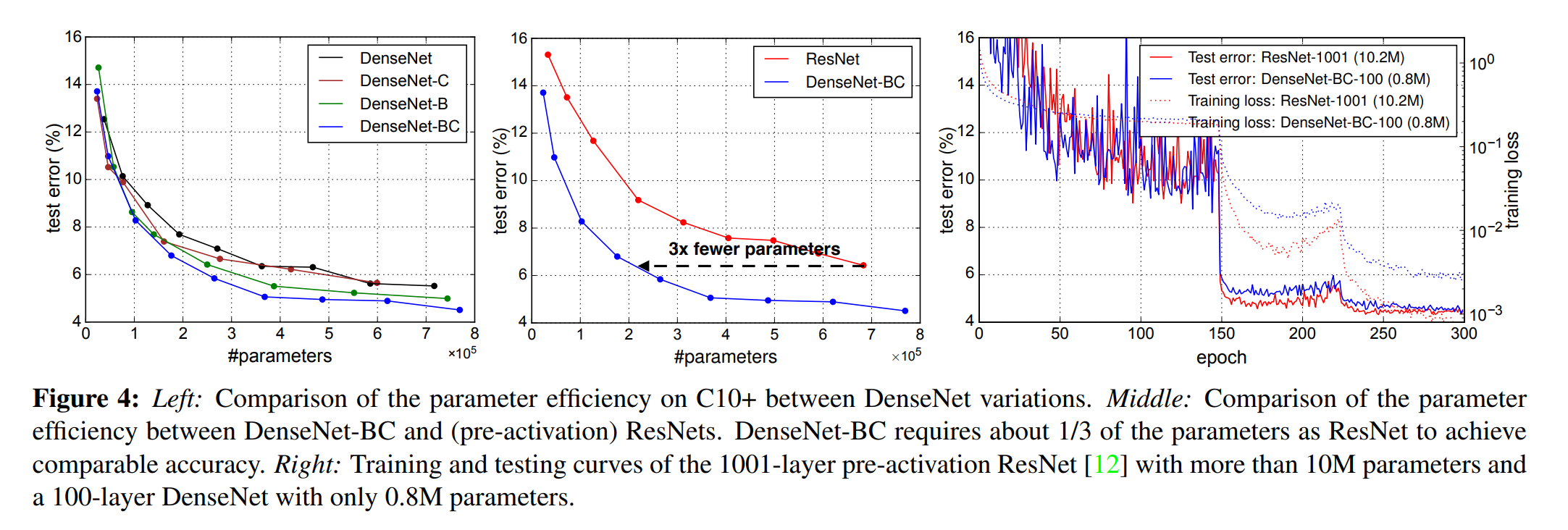
Figure 4 (right panel) shows the training loss and test errors of these two networks on C10+.

• Figure 4은 C10+의 2개의 네트워크에 대한 training loss와 test error를 보여준다.

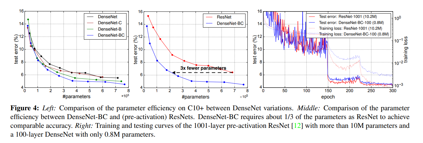
The 1001-layer deep ResNet converges to a lower training loss value but a similar test error.

• 1001-Layer의 깊은 ResNet의 training loss값은 낮게 수렴하지만, test error는 비슷하다.

We analyze this effect in more detail below.

• 이에 대해서는 차후 자세히 분석 예정이다.

Overfitting.

One positive side-effect of the more efficient use of parameters is a tendency of DenseNets to be less prone to overfitting.

• parameter를 더 효율적으로 사용함에 따라 발생하는 긍정적인 부작용 중 하나는 DenseNet이 overfitting 되는 경향이 적다는 것이다.

We observe that on the datasets without data augmentation, the improvements of DenseNet architectures over prior work are particularly pronounced.

• 우리는 데이터 확대가 없는 데이터 세트에서 이전 작업보다 DenseNet 아키텍처의 개선이 특히 두드러진다는 것을 관찰합니다.

On C10, the improvement denotes a 29% relative reduction in error from 7.33% to 5.19%.

• C10에서 error rate가 7.33%에서 5.19%로 상대적으로 29%가량 감소했다.

On C100, the reduction is about 30% from 28.20% to 19.64%.

• C100에서는 28.20%에서 19.64%로 30% 감소했다.

In our experiments, we observed potential overfitting in a single setting: on C10, a 4x growth of parameters produced by increasing k = 12 to k = 24 lead to a modest increase in error from 5.77% to 5.83%.

• 실험에 따르면, single setting에서의 잠재적인 과적합을 확인했다: C10에서 parameter를 4배, k =12에서 k=24로 증가시킴으로써 5.77%에서 5.83%로 약간 증가 했다.

The DenseNet-BC bottleneck and compression layers appear to be an effective way to counter this trend.

• 이를 해결하기 위해서는 DenseNet-BC의 bottleneck과 compression layer가 효과적일 것으로 보인다.

Classification Results on ImageNet

We evaluate DenseNet-BC with different depths and growth rates on the ImageNet classification task, and compare it with state-of-the-art ResNet architectures.

• DenseNet-BC를 네트워크의 깊이와, growth rate를 바꿔가며 ImageNet classification task에서 평가했으며 SOTA인 ResNet과 비교한다.

To ensure a fair comparison between the two architectures, we eliminate all other factors such as differences in data preprocessing and optimization settings by adopting the publicly available Torch implementation for ResNet by [8].

• 두 모델간의 공정한 비교를 위해, Torch implementation된 ResNet을 사용함으로서 데이터 전처리나 최적화 세팅 같이 다를 수 있는 요소들을 모두 제거했다.

We simply replace the ResNet model with the DenseNetBC network, and keep all the experiment settings exactly the same as those used for ResNet.

• 단순히 ResNet 모델을 DenseNet-BC 네트워크로 바꿨으며, 실험 환경은 ResNet과 동일하게 설정했다.

We report the single-crop and 10-crop validation errors of DenseNets on ImageNet in Table 3.

• ImageNet에 DenseNet을 적용한 single-crop과 10-crop validation error 결과는 Table 3와 같다.

Figure 3 shows the single-crop top-1 validation errors of DenseNets and ResNets as a function of the number of parameters (left) and FLOPs (right).

• Figure 3. DenseNet과 ResNets의 single-crop top1 validation error값과의 비교를 위한 그림으로, 왼쪽은 Parameter, 오른쪽은 FLOP에 대한 결과이다.

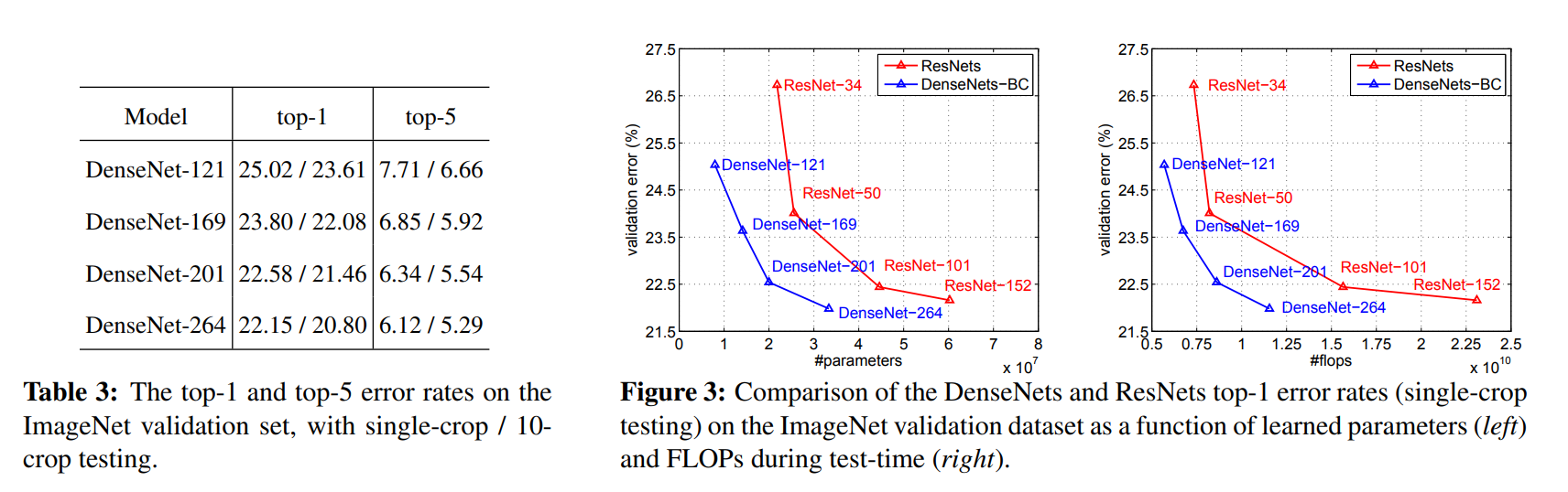
The results presented in the figure reveal that DenseNets perform on par with the state-of-the-art ResNets, whilst requiring significantly fewer parameters and computation to achieve comparable performance.

• 결과를 보면 알 수 있듯, DenseNet의 parameter 수와 computation이 훨씬 적음에도 불구하고, ResNet과 비슷한 성능을 내는 것을 확인할 수 있다.

It is worth noting that our experimental setup implies that we use hyperparameter settings that are optimized for ResNets but not for DenseNets.

• 본 논문에서, 실험 설정이 ResNet에는 최적화되었지만, DenseNet에는 최적화되어 있지 않다는 점 또한 주목할 필요가 있다.

It is conceivable that more extensive hyper-parameter searches may further improve the performance of DenseNet on ImageNet.

• ImageNet에 맞는 DenseNet의 parameter를 보다 최적화한다면, 더 높은 성능을 낼 수 있을 것으로 기대된다.

Discussion

Superficially, DenseNets are quite similar to ResNets: Eq. (2) differs from Eq. (1) only in that the inputs to \(H_l(\cdot)\) are concatenated instead of summed.

• Eq(2)(DenseNet)는 Eq(1)(ResNet)와 다른데, 채널이 더 해지는 것 대신에 concat된다는 점 빼고고는 표면적으로 보았을 때, DenseNet의 구조는 ResNet과 상당히 유사하다.

However, the implications of this seemingly small modification lead to substantially different behaviors of the two network architectures.

• 하지만, 두 구조간의 작은 차이는 실질적으로 두 네트워크 구조 간의 아주 큰 차이로 이어진다.

Model compactness.

As a direct consequence of the input concatenation, the feature-maps learned by any of the DenseNet layers can be accessed by all subsequent layers.

• input concatenation의 직접적인 결과로, DenseNet에서 학습된 feature map들은 모든 subsequent Layer(그 이후의 layer)에 접근 가능하다.

This encourages feature reuse throughout the network, and leads to more compact models.

• 이는 네트워크 전체의 feature 재사용성을 높이고, 보다 compact한 모델이 되도록 한다.

The left two plots in Figure 4 show the result of an experiment that aims to compare the parameter efficiency of all variants of DenseNets (left) and also a comparable ResNet architecture (middle).

왼쪽 그래프는 DenseNet의 parameter efficiency를 비교하는 그래프, 가운데 그래프는 ResNet 구조와 DenseNet을 비교하는 그래프이다.

We train multiple small networks with varying depths on C10+ and plot their test accuracies as a function of network parameters.

C10+에서 다양한 깊이의 여러 소규모 네트워크들을 train하고, network parameter들의 function으로 test 정확도를 점으로 나타냈다.

In comparison with other popular network architectures, such as AlexNet [16] or VGG-net [29], ResNets with pre-activation use fewer parameters while typically achieving better results [12].

AlexNet이나 VGG-net과 같은 여러 유명한 네트워크 구조와 비교했을 때, pre-activation된 ResNet은 적은 parameter에도 일반적으로 더 나은 결과를 냈다.

Hence, we compare DenseNet (k = 12) against this architecture.

• 따라서 DenseNet(k=12)를 이 아키텍처와 비교한다.

The training setting for DenseNet is kept the same as in the previous section.

• DenseNet에 대한 training setting은 이전 섹션과 동일하게 유지된다.

The graph shows that DenseNet-BC is consistently the most parameter efficient variant of DenseNet.

• 그래프는 상에서 DenseNet-BC가 가장 효율적으로 paramter가 구성되어있다.

Further, to achieve the same level of accuracy, DenseNet-BC only requires around 1/3 of the parameters of ResNets (middle plot).

• 더욱이 동일한 수준의 정확도를 달성하는데 DenseNet-BC는 ResNet의 약 1/3 정도의 parameter만 이용했다.(가운데 표)

This result is in line with the results on ImageNet we presented in Figure 3.

• Figure 3에 ImageNet에 대한 결과를 타나낸다.

The right plot in Figure 4 shows that a DenseNet-BC with only 0.8M trainable parameters is able to achieve comparable accuracy as the 1001-layer (pre-activation) ResNet [12] with 10.2M parameters.

• Figure 4의 오른쪽 도표에서 보여주듯이 0.8M개의 parameter를 사용하는 DenseNet-BC가 10.2M의 parameter를 사용하는 1001-layer ResNet과 유사한 성능을 보여준다.

Implicit Deep Supervision.

One explanation for the improved accuracy of dense convolutional networks may be that individual layers receive additional supervision from the loss function through the shorter connections.

dense convolutional network의 accuracy가 향상되는 이유는 각각의 Layer들이 short connection을 통해 loss function의 추가적인 supervision(backpropagation시 직접적으로 영향)을 받기 때문이다.

One can interpret DenseNets to perform a kind of “deep supervision”.

DenseNet을 이용해 일종의 "Deep supervision"을 수행할 수 있다.

The benefits of deep supervision have previously been shown in deeply-supervised nets (DSN; [20]), which have classifiers attached to every hidden layer, enforcing the intermediate layers to learn discriminative features.

• Deep supervision의 이점은 이미 deeply-supervised nets(DSN)에서 증명된 바 있다, 모든 hidden Layer에 classifier가 더해지며, intermediate Layer들이 보다 차별적인 특징을 학습하도록 한다.

DenseNets perform a similar deep supervision in an implicit fashion: a single classifier on top of the network provides direct supervision to all layers through at most two or three transition layers.

• DenseNet은 implicit(암묵적)한 방식으로 위와 유사한 Deep supervision을 수행한다 : 네트워크 상단의 single classifier는 최대 2~3개의 transition Layer를 통해 모든 Layer를 직접적으로 supervision한다.

However, the loss function and gradient of DenseNets are substantially less complicated, as the same loss function is shared between all layers.

• 하지만 DenseNet의 loss function과 gradient의 경우, 모든 Layer에서 같은 loss function을 공유하기 때문에 훨씬 덜 복잡하다.

Stochastic vs. deterministic connection.

There is an interesting connection between dense convolutional networks and stochastic depth regularization of residual networks [13].

• dense convolutional network와 residual network의 stochastic depth regularization사이에는

흥미로운 connection이 하나 있다.

In stochastic depth, layers in residual networks are randomly dropped, which creates direct connections be-tween the surrounding layers.

• stochastic depth에서, residual network의 Layer들은 랜덤하게 drop되어 주변 Layer들 간의 direct connection이 생성된다.

As the pooling layers are never dropped, the network results in a similar connectivity pattern as DenseNet.

• pooling Layer는 drop하지 않기 때문에 네트워크는 DenseNet과 유사한 connectivity pattern을 갖는다.

Although the methods are ultimately quite different, the DenseNet interpretation of stochastic depth may provide insights into the success of this regularizer.

• 방법은 궁극적으로 다를지 몰라도, stochastic depth에 대한 DenseNet interpretation은 정규화의 성공에 대한 통찰력을 제공한다.

Feature Reuse.

By design, DenseNets allow layers access to feature-maps from all of its preceding layers (although sometimes through transition layers).

• DenseNet은 현재 Layer가 이전의 모든 Layer들의 feature map에 접근할 수 있도록 설계되었다.

We conduct an experiment to investigate if a trained network takes advantage of this opportunity.

• 본 논문에서는 train된 네트워크가 이러한 기회를 잘 활용하는지 조사하기 위해 다음과 같은 실험을 수행했다.

We first train a DenseNet on C10+ with L = 40 and k = 12.

• 먼저, C10+, k = 12, L = 40인 DenseNet을 훈련시켰다.

For each convolutional layer \(l\) within a block, we compute the average (absolute) weight assigned to connections with layer \(s\).

• 각 블록 내의 convolutional Layer 'l'에 대해, Layer 's'와의 연결에 할당된 average weight를 계산했다.

Figure 5 shows a heat-map for all three dense blocks.

• Figure 5. 는 모든 3개의 dense block에 대한 heat-map을 나타낸 그림이다.

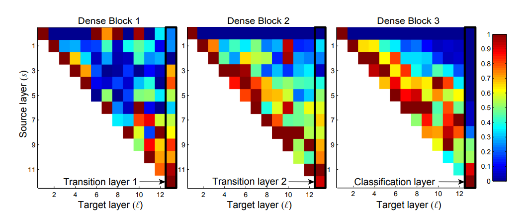
The average absolute weight serves as a surrogate for the dependency of a convolutional layer on its preceding layers.

• average absolute weight란, 이전 Layer에서 Convolution Layer에 대한 의존성에 대한 정도이다.

A red dot in position \((l,s)\) indicates that the layer \(l\) makes, on average, strong use of feature-maps produced s-layers before.

• 위 그림에서 빨간색 점\((l,s)\)은 Layer '\(l\)'이 이전 Layer '\(s\)'에서 생성된 feature-map을 많이 사용한다는 것을 나타낸다.

Conclusion

We proposed a new convolutional network architecture, which we refer to as Dense Convolutional Network(DenseNet).

• 본 논문에서는 Dense Convolutional Network, 일명 DenseNet이라고 불리는 새로운 Convolutional Network 구조에 대해 소개했다.

It introduces direct connections between any two layers with the same feature-map size.

• 같은 feature map size를 가진 어떤 2개의 Layer들에 대한 direct connection에 대해 소개했다.

We showed that DenseNets scale naturally to hundreds of layers, while exhibiting no optimization difficulties.

• optimization 어려움없이 Layer의 규모를 많이 늘려나갈 수 있다는 것 또한 증명했다.

In our experiments, DenseNets tend to yield consistent improvement in accuracy with growing number of parameters, without any signs of performance degradation or overfitting.

• 본 논문의 실험에서, DenseNet은 성능저하나 overfitting없이 parameter의 개수가 증가할수록 정확도가 향상되는 모습을 보였다.

Under multiple settings, it achieved state-of-the-art results across several highly competitive datasets.

• 다양한 설정에서도 다른 기존 결과들에 비해 놀라운 성과를 보여줬다.

Moreover, DenseNets require substantially fewer parameters and less computation to achieve state-of-the-art performances.

• 심지어는 다른 구조들에 비해 상당히 적은 parameter 개수와 연산량으로 더 좋은 결과를 냈다.

Because we adopted hyperparameter settings optimized for residual networks in our study, we believe that further gains in accuracy of DenseNets may be obtained by more detailed tuning of hyperparameters and learning rate schedules.

• 본 논문에서 DenseNet의 parameter들은 ResNet환경에 맞게 setting되었는데, hyper parameter tunning과 learning rate 스케줄을 개선하면 더 좋은 결과가 나올 것으로 예상하고 있다.

Whilst following a simple connectivity rule, DenseNets naturally integrate the properties of identity mappings, deep supervision, and diversified depth.

• DenseNet은 모든 Layer들을 연결한다는 간단한 connectivity rule을 따르면서도, identity mapping, deep supervision, diversified depth 등의 특징을 모두 실현시켰다.

They allow feature reuse throughout the networks and can consequently learn more compact and, according to our experiments, more accurate models.

• DenseNet 구조는 네트워크 전체에서 feature 재사용을 더 용이하게 하고, model을 더 compact하게 만들었다.

Because of their compact internal representations and reduced feature redundancy, DenseNets may be good feature extractors for various computer vision tasks that build on convolutional features, e.g., [4, 5].

• DenseNet은 compact한 internal representations, 중복 feature 감소라는 장점을 통해 다양한 컴퓨터 비전 분야에서 훌륭한 feature extractor로 자리잡을 것이다.

We plan to study such feature transfer with DenseNets in future work.

• DenseNets를 사용하여 향후 feature transfer를 연구할 계획이다.

[reference]

https://arxiv.org/pdf/1608.06993.pdf