
서론
이 장은 ConvNet의 장점을 유지하면서 backbone의 ResNet을 개선한 모델인 ConvNeXt에 대해서 소개한다.
목차
- Training Techniques
- Modernizing a ConvNet: a Roadmap
- Macro Design (1)
- ResNeXt
- Inverted Bottleneck
- Large Kernel Size
- Micro Design (2)
- Fewer activations
- Experiments
- Concolusion
Training Techniques
- Original 90 epochs → Extended to 300 epochs
- Use AdamW Optimizer
- Data Augmentation
- Mixup, Cutmix, RandAugment, Random Erasing
- Regularization
- Stochas-tic Depth, Label Smoothing
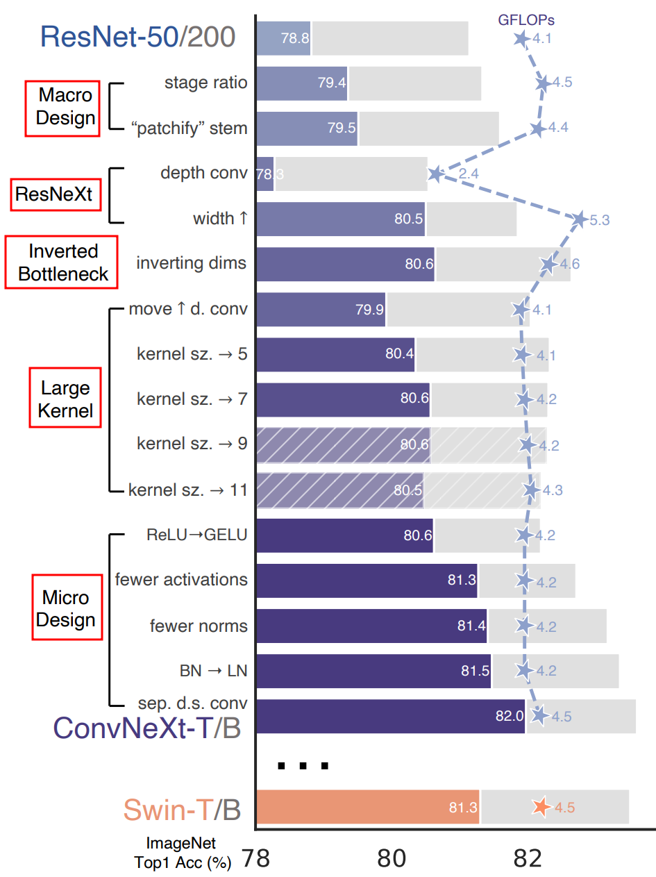
- performance of the ResNet-50 Model from 76.1% to 78.8%
Modernizing a ConvNet: a Roadmap
ConvNet을 어떻게 개선했는지에 대한 로드맵이다. 각 단계별로 어떤 것들이 적용됐는지 알아보겠다.
Macro Design (1)
Changing stage compute ratio
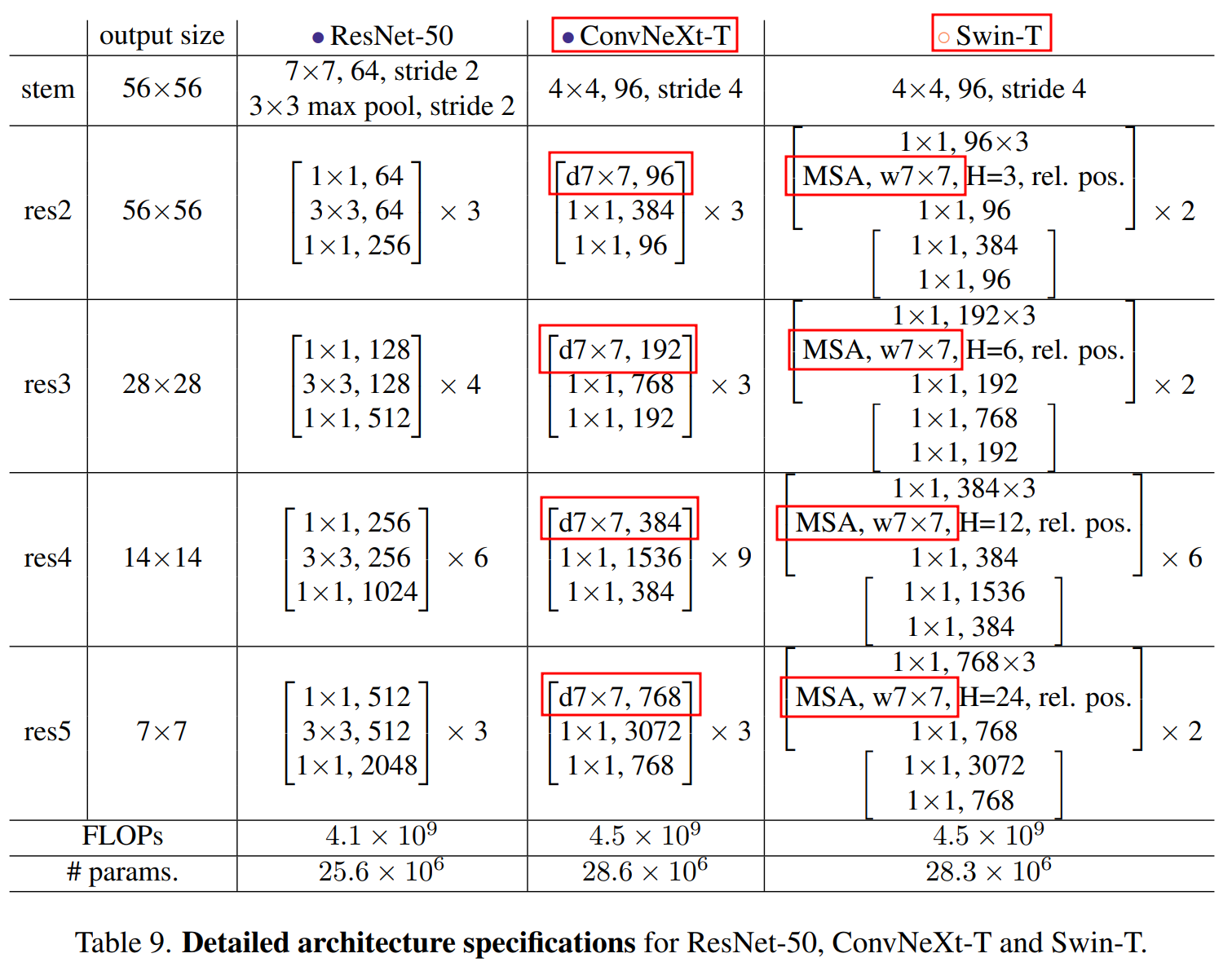
- 기존 ResNet-50은 각 Block (3→4→6→3) 에서 3→3→9→3 (1:1:3:1)로 구성
- Swin-T가 2→2→6→2(1:1:3:1) 로 구성되어 있음
This improves the model accuracy from 78.8% to 79.4%.
Changing stem to “Patchify”
- Swin-T의 patch size가 4와 같이 ResNet에도 4x4 kernel size, stride 4를 통해 patchify 수행
The accuracy has changed from 79.4% to 79.5%.
ResNeXt
- Depthwise Convolution 사용(Xception에서 제안됨)
- 연산량(FLOPs)를 줄이고 capacity 유지
- 채널 별로 가중합을 한다는 관점에서 self-attention과 유사
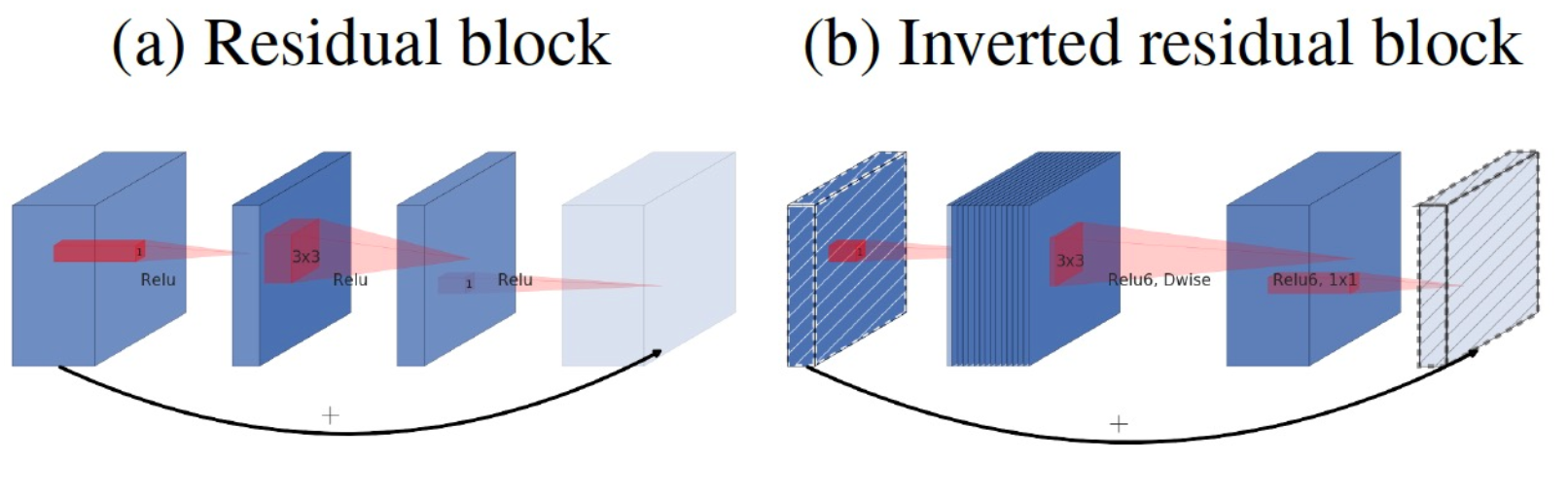
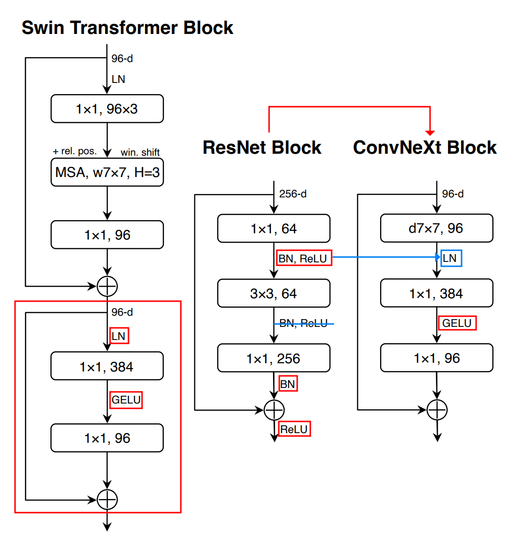
Inverted Bottleneck
- MobileNetV2의 inverted residuals 방법을 사용(메모리 효율적 [Figure3. a→b])
- (a) 1x1, 384 input→ 96 →1x1, 384 output
- (b) 1x1 96 input→ 384 → 1x1, 96 output
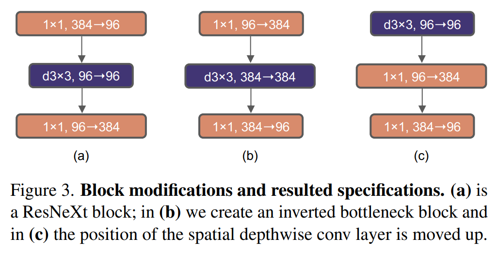
- Large kernel size를 위해서 3x3 kernel을 위쪽으로 layer 이동([Figure3. b→c])
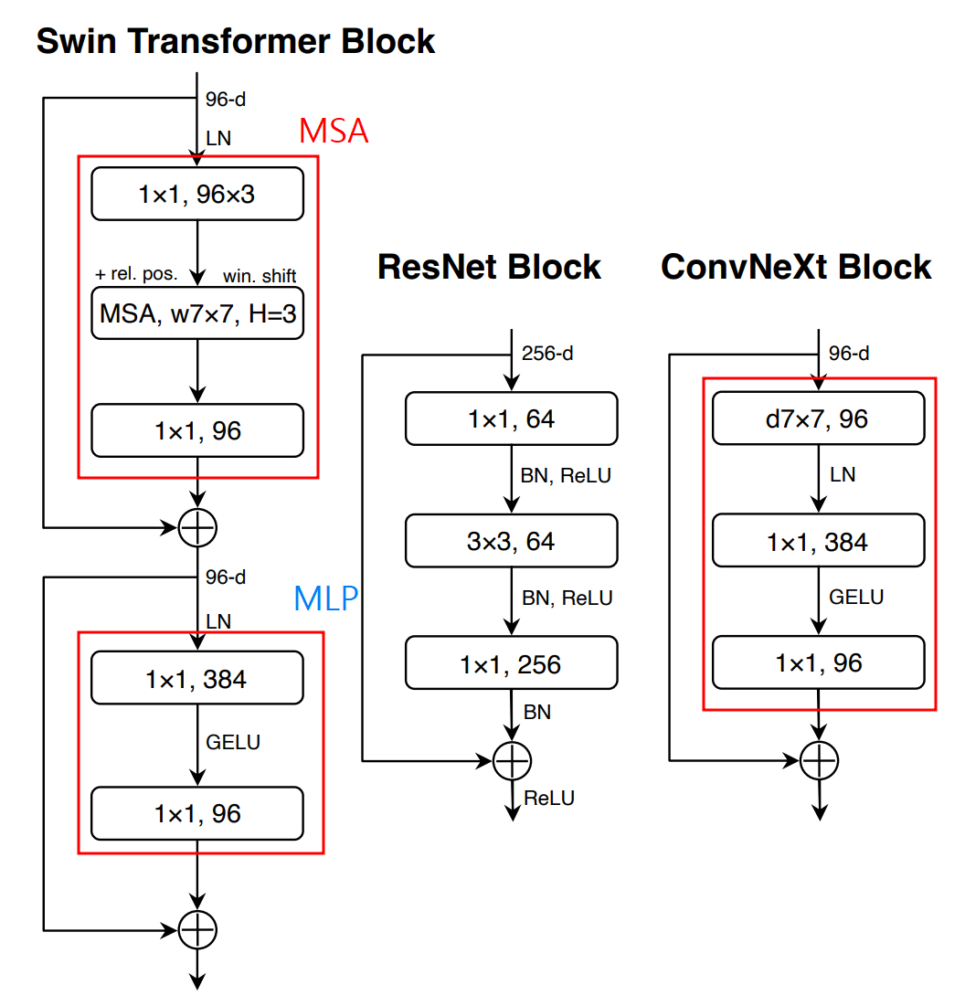
- Swin-T 동일한 구조
Large Kernel Size
Increasing he kernel size
- Swin-T에서 Window size가 7x7이 사용되어 지므로 ConvNeXt에서도 7x7 depthwise conv사용
Micro Design (2)
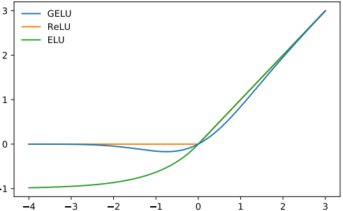
ReLU → GELU (Gaussian Error Linear Unit)
- 최신 Trend 모델들인 BERT, GPT-2 등 Relu대신 Gelu사용
Fewer activations
- Swin-T 에서는 MLP Block에 하나의 Activation Function만을 가지고 있음
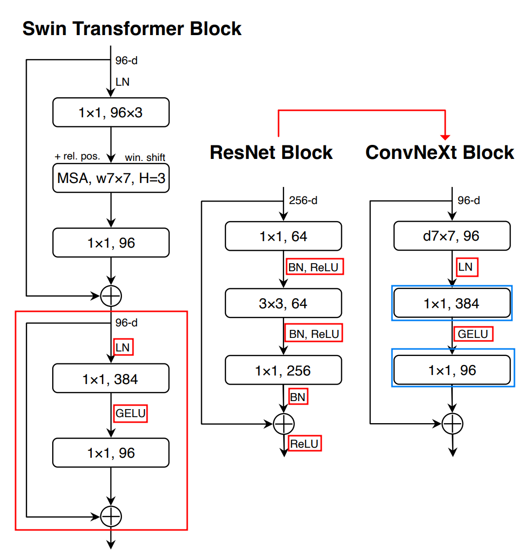
- 두 개의 1x1 layer(conv) 사이에 있는 layer를 제외하고 모든 GELU layer를 제거
We eliminate all GELU layers from the residual block except for one between two 1x1 layers
Fewer Normalization Layers
- 두개의 Batch Normalization을 1x1 Conv 이전 layer(즉, d7x7 layer 출력 이후)에 하나만 사용
We remove two BatchNorm(BN) layers, leaving only one BN layer before the conv 1x1 layers.
- single BN layer(before conv 1x1 layer)→ Layer Normalization으로 변경
Seperate Downsampling layers
- 매번 Convolution Layer 이후 down-sampleing → Stage 마다 down-sampling
Experiments
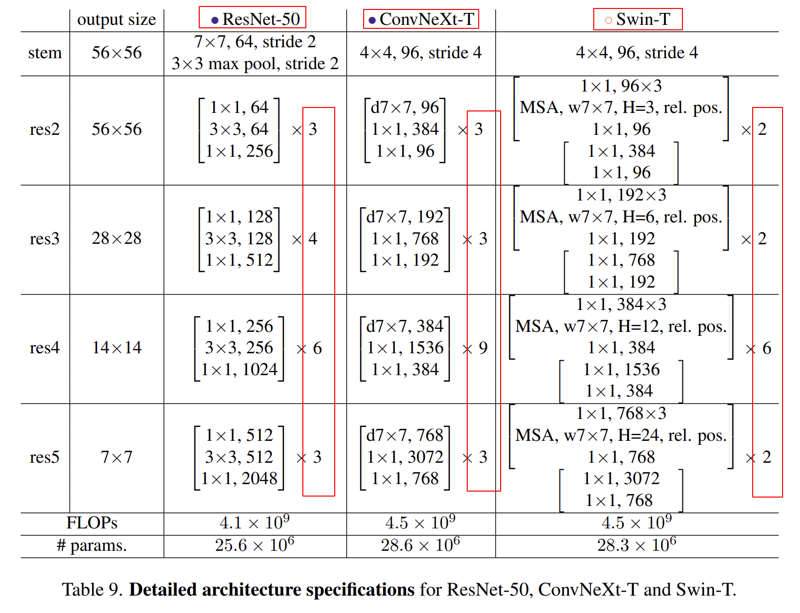
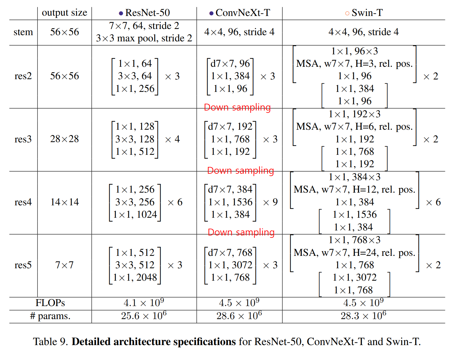
Swin-T와 비슷하게 여러 Dimension & Block으로 모델 구성
- ConvNeXt-T: C = (96, 192, 384, 768), B = (3, 3, 9, 3)
- ConvNeXt-S: C = (96, 192, 384, 768), B = (3, 3, 27, 3)
- ConvNeXt-B: C = (128, 256, 512, 1024), B = (3, 3, 27, 3)
- ConvNeXt-L: C = (192, 384, 768, 1536), B = (3, 3, 27, 3)
- ConvNeXt-XL: C = (256, 512, 1024, 2048), B = (3, 3, 27, 3)
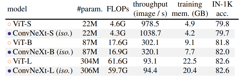
Isotropic ConvNeXt vs ViT
- ViT와 동일하게 Down-sampling없이 비교하였다.
- 동일한 성능 대비 적은 연산량(FLOPs)을 보인다.
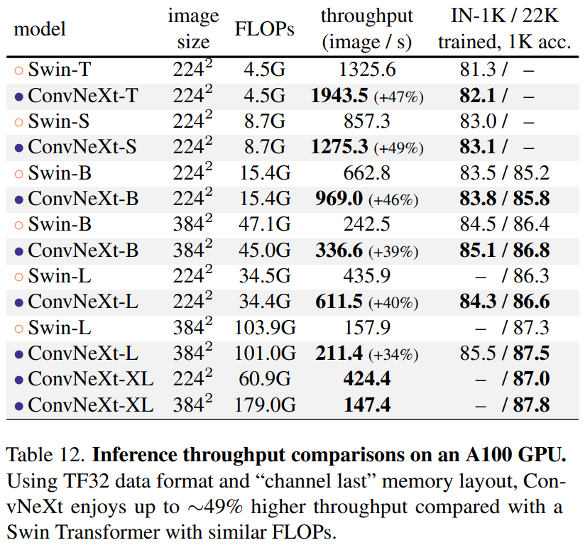
Inference
- Swin-T에 비해 ConvNeXt의 추론 속도가 빠르다.
Concolusion
- In the 2020s, Swin Transformers overtake ConvNets as the favored choice for generic vision backbones.
- We propose ConvNeXts can compete with Swin-T, while retaining the simplicity and efficiency of standard ConvNets.
- Our ConvNeXt model itself is not completely new
- We hope that the new results reported in this study will challenge several widely held views and prompt people to rethink the importance of convolution in computer vision
https://coding-yoon.tistory.com/122
https://blog.kubwa.co.kr/%EB%85%BC%EB%AC%B8%EB%A6%AC%EB%B7%B0-a-convnet-for-the-2020s-9b45ac666d04
Comment